We teach the robot to cook pizza. Part 2: Neural Network Contest
Content
In the last part, we managed to parse the Dodo-Pizza website and load the data on the ingredients, and most importantly, the pizza photos. In total, we had 20 pizzas at our disposal. Of course, it will not be possible to generate training data from just 20 pictures. However, you can use the axial symmetry of the pizza: by rotating the image in one-degree increments and vertical reflection, you can turn one photo into a set of 720 images. Too little, but still try.
Let's try to train the Conditional Variational Autoencoder, and then move on to what it all was for — generative adversary neural networks (Generative Adversarial Networks).
CVAE - conditional variational autoencoder
For proceedings with autoencoders, an excellent series of articles will help:
- Autoencoders in Keras, Part 3: Variational autoencoders (VAE)
- Autoencoders in Keras, Part 4: Conditional VAE
I strongly recommend reading.
Here we go straight to the point.
The difference between CVAE and VAE is that we need to input both the encoder and the decoder, additionally submit another label. In our case, the label will be the recipe vector that we get from OneHotEncoder.
However, there is a nuance - and at what point does it make sense to submit our tag?
I tried two methods:
- at the end - after all convolutions - before a fully connected layer
- at the beginning - after the first convolution - is added as an additional channel
In principle, both methods have the right to exist. It seems logical that if you add a label at the end, it will be attached to higher-level image features. And vice versa - if you add it at the beginning, it will be tied to lower-level features. Let's try to compare both ways.
Recall that the recipe consists of a maximum of 9 ingredients. And there are only 28 of them. It turns out that the recipe code will be a 9x29 matrix, and if you pull it out, you get a 261-dimensional vector.
For an image size of 32x32, choose the size of the hidden space is equal to 512.
You can choose less, but as will be seen later, this leads to a more blurred result.
The code for the encoder with the first method of adding a tag is after all convolutions:
def create_conv_cvae(channels, height, width, code_h, code_w): input_img = Input(shape=(channels, height, width)) input_code = Input(shape=(code_h, code_w)) flatten_code = Flatten()(input_code) latent_dim = 512 m_height, m_width = int(height/4), int(width/4) x = Conv2D(32, (3, 3), activation='relu', padding='same')(input_img) x = MaxPooling2D(pool_size=(2, 2), padding='same')(x) x = Conv2D(16, (3, 3), activation='relu', padding='same')(x) x = MaxPooling2D(pool_size=(2, 2), padding='same')(x) flatten_img_features = Flatten()(x) x = concatenate([flatten_img_features, flatten_code]) x = Dense(1024, activation='relu')(x) z_mean = Dense(latent_dim)(x) z_log_var = Dense(latent_dim)(x) The code for the encoder with the second labeling method - after the first convolution - as an additional channel:
def create_conv_cvae2(channels, height, width, code_h, code_w): input_img = Input(shape=(channels, height, width)) input_code = Input(shape=(code_h, code_w)) flatten_code = Flatten()(input_code) latent_dim = 512 m_height, m_width = int(height/4), int(width/4) def add_units_to_conv2d(conv2, units): dim1 = K.int_shape(conv2)[2] dim2 = K.int_shape(conv2)[3] dimc = K.int_shape(units)[1] repeat_n = dim1*dim2 count = int( dim1*dim2 / dimc) units_repeat = RepeatVector(count+1)(units) #print('K.int_shape(units_repeat): ', K.int_shape(units_repeat)) units_repeat = Flatten()(units_repeat) # cut only needed lehgth of code units_repeat = Lambda(lambda x: x[:,:dim1*dim2], output_shape=(dim1*dim2,))(units_repeat) units_repeat = Reshape((1, dim1, dim2))(units_repeat) return concatenate([conv2, units_repeat], axis=1) x = Conv2D(32, (3, 3), activation='relu', padding='same')(input_img) x = add_units_to_conv2d(x, flatten_code) #print('K.int_shape(x): ', K.int_shape(x)) # size here: (17, 32, 32) x = MaxPooling2D(pool_size=(2, 2), padding='same')(x) x = Conv2D(16, (3, 3), activation='relu', padding='same')(x) x = MaxPooling2D(pool_size=(2, 2), padding='same')(x) x = Flatten()(x) x = Dense(1024, activation='relu')(x) z_mean = Dense(latent_dim)(x) z_log_var = Dense(latent_dim)(x) The decoder code in both cases is the same - the label is added at the very beginning.
z = Input(shape=(latent_dim, )) input_code_d = Input(shape=(code_h, code_w)) flatten_code_d = Flatten()(input_code_d) x = concatenate([z, flatten_code_d]) x = Dense(1024)(x) x = Dense(16*m_height*m_width)(x) x = Reshape((16, m_height, m_width))(x) x = Conv2D(16, (3, 3), activation='relu', padding='same')(x) x = UpSampling2D((2, 2))(x) x = Conv2D(32, (3, 3), activation='relu', padding='same')(x) x = UpSampling2D((2, 2))(x) decoded = Conv2D(channels, (3, 3), activation='sigmoid', padding='same')(x) Number of network parameters:
- 4'221'987
- 3'954'867
The speed of learning for one era:
- 60 sec
- 63 seconds
Result after 40 epochs of study:
- loss: -0.3232 val_loss: -0.3164
- loss: -0.3245 val_loss: -0.3191
As you can see, the second method requires less memory for the INS, gives a better result, but takes a little more time to learn.
It remains to visually compare the results of the work.
- Original image (32x32)
- The result of the work is the first method (latent_dim = 64)
- The result of the work is the first method (latent_dim = 512)
- The result of the work is the second method (latent_dim = 512)


Now let's see how the pizza transfer application looks like when the pizza is encoded with the original recipe and decoded with another.
i = 0 for label in labels: i += 1 lbls = [] for j in range(batch_size): lbls.append(label) lbls = np.array(lbls, dtype=np.float32) print(i, lbls.shape) stt_imgs = stt.predict([orig_images, orig_labels, lbls], batch_size=batch_size) save_images(stt_imgs, dst='temp/cvae_stt', comment='_'+str(i)) The result of the work transfer style (the second encoding method):

GAN - Generative Competitive Network
I did not manage to find the well-established Russian-language names of such networks.
Options:
- generative competition networks
- spawning networks
- spawning networks
I like it more:
- generative competitive networks
With the theory of the work of GAN again, an excellent series of articles will help:
- Autoencoders in Keras, Part 5: GAN (Generative Adversarial Networks) and tensorflow
- Autoencoders in Keras, Part 6: VAE + GAN
And for a deeper understanding - the latest article in the blog ODS: Neural network game in imitation
However, starting to understand and try to independently implement the generative neural network - I was faced with some difficulties. For example, there were moments when the generator gave out really psychedelic pictures.
Different examples helped to understand the implementation:
MNIST Generative Adversarial Model in Keras ( mnist_gan.py ),
Architecture recommendations from the end of 2015 article from facebook research about DCGAN (Deep Convolutional GAN):
Unsupervised Representation Learning with Deep Convolutional Generative Adversarial Networks
as well as a set of recommendations to make GAN work:
How to Train a GAN? Tips and tricks to make GANs work .
Constructing a GAN:
def make_trainable(net, val): net.trainable = val for l in net.layers: l.trainable = val def create_gan(channels, height, width): input_img = Input(shape=(channels, height, width)) m_height, m_width = int(height/8), int(width/8) # generator z = Input(shape=(latent_dim, )) x = Dense(256*m_height*m_width)(z) #x = BatchNormalization()(x) x = Activation('relu')(x) #x = Dropout(0.3)(x) x = Reshape((256, m_height, m_width))(x) x = Conv2DTranspose(256, kernel_size=(5, 5), strides=(2, 2), padding='same', activation='relu')(x) x = Conv2DTranspose(128, kernel_size=(5, 5), strides=(2, 2), padding='same', activation='relu')(x) x = Conv2DTranspose(64, kernel_size=(5, 5), strides=(2, 2), padding='same', activation='relu')(x) x = Conv2D(channels, (5, 5), padding='same')(x) g = Activation('tanh')(x) generator = Model(z, g, name='Generator') # discriminator x = Conv2D(128, (5, 5), padding='same')(input_img) #x = BatchNormalization()(x) x = LeakyReLU()(x) #x = Dropout(0.3)(x) x = MaxPooling2D(pool_size=(2, 2), padding='same')(x) x = Conv2D(256, (5, 5), padding='same')(x) x = LeakyReLU()(x) x = MaxPooling2D(pool_size=(2, 2), padding='same')(x) x = Conv2D(512, (5, 5), padding='same')(x) x = LeakyReLU()(x) x = MaxPooling2D(pool_size=(2, 2), padding='same')(x) x = Flatten()(x) x = Dense(2048)(x) x = LeakyReLU()(x) x = Dense(1)(x) d = Activation('sigmoid')(x) discriminator = Model(input_img, d, name='Discriminator') gan = Sequential() gan.add(generator) make_trainable(discriminator, False) #discriminator.trainable = False gan.add(discriminator) return generator, discriminator, gan gan_gen, gan_ds, gan = create_gan(channels, height, width) gan_gen.summary() gan_ds.summary() gan.summary() opt = Adam(lr=1e-3) gopt = Adam(lr=1e-4) dopt = Adam(lr=1e-4) gan_gen.compile(loss='binary_crossentropy', optimizer=gopt) gan.compile(loss='binary_crossentropy', optimizer=opt) make_trainable(gan_ds, True) gan_ds.compile(loss='binary_crossentropy', optimizer=dopt) As you can see, the discriminator is the usual binary classifier, which produces:
1 - for real pictures,
0 - for fake.
Learning procedure:
- we receive a portion of real pictures
- we generate noise on the basis of which the generator generates pictures
- we form a batch for learning the discriminator, which consists of real images (they are assigned the label 1) and fakes from the generator (label 0)
- we train the discriminator
- we train the GAN (the generator is trained in it, because the discriminator’s training is turned off), giving noise to the input and waiting for the 1 mark at the output.
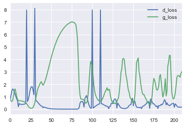
for epoch in range(epochs): print('Epoch {} from {} ...'.format(epoch, epochs)) n = x_train.shape[0] image_batch = x_train[np.random.randint(0, n, size=batch_size),:,:,:] noise_gen = np.random.uniform(-1, 1, size=[batch_size, latent_dim]) generated_images = gan_gen.predict(noise_gen, batch_size=batch_size) if epoch % 10 == 0: print('Save gens ...') save_images(generated_images) gan_gen.save_weights('temp/gan_gen_weights_'+str(height)+'.h5', True) gan_ds.save_weights('temp/gan_ds_weights_'+str(height)+'.h5', True) # save loss df = pd.DataFrame( {'d_loss': d_loss, 'g_loss': g_loss} ) df.to_csv('temp/gan_loss.csv', index=False) x_train2 = np.concatenate( (image_batch, generated_images) ) y_tr2 = np.zeros( [2*batch_size, 1] ) y_tr2[:batch_size] = 1 d_history = gan_ds.train_on_batch(x_train2, y_tr2) print('d:', d_history) d_loss.append( d_history ) noise_gen = np.random.uniform(-1, 1, size=[batch_size, latent_dim]) g_history = gan.train_on_batch(noise_gen, np.ones([batch_size, 1])) print('g:', g_history) g_loss.append( g_history ) Please note that, unlike a variational autoencoder, the real images are not used for the generator training, but only the discriminator mark. Those. the generator is trained on error gradients from the discriminator.
The most interesting thing is that the name of competitive networks is not for a beautiful word - they really try and even follow the testimony of the losses of the discriminator and generator.
If you look at the loss curves, you can see that the discriminator quickly learns to distinguish the real picture from the original garbage emitted by the generator, but then the curves begin to oscillate — the generator learns to generate an increasingly appropriate image.
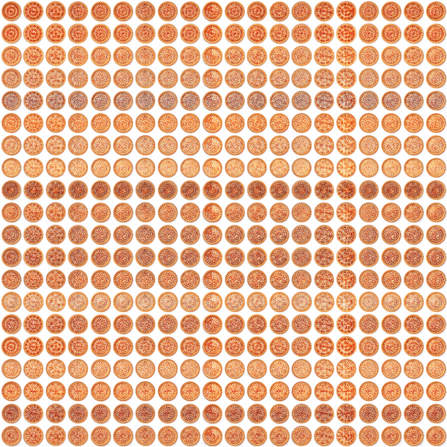
gif-ka showing the process of learning the generator (32x32) on one pizza (the first pizza on the list is Double pepperoni):

As expected, the result of the GAN operation, compared with the variational encoder, gives a clearer image.
CVAE + GAN - conditional variational avtoenkorder and generative adversarial network
It remains to combine CVAE and GAN together to get the best from both networks. The basis of the union is a simple idea - the VAE decoder performs exactly the same function as the GAN generator, but they perform and learn it in different ways.
In addition to what is not completely clear, how to make it all work together, it was also not clear to me that you can use different loss functions in Keras. The examples on the githaba helped to understand this question:
Thus, the application of various loss functions in Keras can be implemented by adding your own layer ( Writing your own Keras layers ), in the call () method of which you can implement the required calculation logic with a subsequent call to the add_loss () method.
Example:
class DiscriminatorLossLayer(Layer): __name__ = 'discriminator_loss_layer' def __init__(self, **kwargs): self.is_placeholder = True super(DiscriminatorLossLayer, self).__init__(**kwargs) def lossfun(self, y_real, y_fake_f, y_fake_p): y_pos = K.ones_like(y_real) y_neg = K.zeros_like(y_real) loss_real = keras.metrics.binary_crossentropy(y_pos, y_real) loss_fake_f = keras.metrics.binary_crossentropy(y_neg, y_fake_f) loss_fake_p = keras.metrics.binary_crossentropy(y_neg, y_fake_p) return K.mean(loss_real + loss_fake_f + loss_fake_p) def call(self, inputs): y_real = inputs[0] y_fake_f = inputs[1] y_fake_p = inputs[2] loss = self.lossfun(y_real, y_fake_f, y_fake_p) self.add_loss(loss, inputs=inputs) return y_real gif-ka showing the learning process (64x64):

The result of the work transfer style:
And now the fun part!
Actually for the sake of what it all was started - the generation of pizza for the selected ingredients.
Let's look at pizza with a recipe consisting of one ingredient (ie, with codes from 1 to 27):
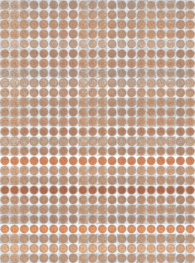
As expected, only pizzas with the most popular ingredients 24, 20, 17 (tomatoes, pepperoni, mozzarella) look more or less - all other options are something dull with round shapes and incomprehensible gray spots in which only on request You can try to guess something.
Conclusion
In general, the experiment can be considered partially successful. However, even on such a toy example, one feels that the pathos expression: “data is new oil” - has a right to exist, especially with regard to machine learning.
After all, the quality of the application based on machine learning, depends primarily on the quality and quantity of data.
Generative networks are really very interesting and, it seems that in the foreseeable future we will see many different examples of their use.
By the way, a good question arises: if the rights to photos belong to their creator, then who owns the rights to the picture that the neural network creates?
Thank you very much for your attention!
Nb. When writing this article - not a single pizza has suffered.
Links
- Autoencoders in Keras, Part 3: Variational autoencoders (VAE)
- Autoencoders in Keras, Part 4: Conditional VAE
- Autoencoders in Keras, Part 5: GAN (Generative Adversarial Networks) and tensorflow
- Autoencoders in Keras, Part 6: VAE + GAN
- Deep Convolutional GANs (DCGAN): Unsupervised Representation Learning with Deep Convolutional Generative Adversarial Networks
- How to Train a GAN? Tips and tricks to make GANs work
- Keras VAEs and GANs
- MNIST Generative Adversarial Model in Keras ( mnist_gan.py )
- Generative Adversarial Networks Part 2 - Implementation with Keras 2.0
- Generative Adversarial Networks with Keras
- GAN by Example using Keras on Tensorflow Backend
- Keras implementation of Deep Convolutional Generative Adversarial Networks (DCGAN)
- Generative models from OpenAI
- Neural network imitation game
')
Source: https://habr.com/ru/post/337398/
All Articles