Shazam: music recognition algorithms, signatures, data processing
An almost forgotten song played in the restaurant. You listened to her in the distant past. How many touching memories can cause chords and words ... You desperately want to listen to this song again, but its name completely disappeared from your head! How to be? Fortunately, in our fantastic high-tech world there is an answer to this question.
You have a smartphone in your pocket, which has a program for recognizing music. This program is your savior. In order to find out the name of the song, you will not have to walk from corner to corner in an attempt to extract the cherished line from your own memory. And after all not the fact that it will turn out. The program, if you let it “listen” to the music, immediately reports the name of the composition. After that, you can listen to the sweet heart sounds again and again. Until they become one with you, or - until you get tired of all this.
Mobile technologies and incredible progress in the field of sound processing give algorithm developers the ability to create music recognition applications. One of the most popular solutions of this kind is called Shazam . If you give it 20 seconds of sound, no matter whether it is a piece of an intro, chorus or part of the main motive, Shazam will create a signature code, check the database and use its own music recognition algorithm to give the name of the piece.
')
How does all this work?
The description of the basic Shazam algorithm in 2003 was published by its creator, Avery Li-Chung Wang (Avery Li-Chung Wang). In this article, we will examine in detail the basics of the Shazam music recognition algorithm.
What is sound, really? Maybe it is some mysterious bodiless substance that penetrates our ears and allows us to hear?
Of course, everything is not so mysterious. It has long been known that sound is mechanical vibrations that propagate in solid, liquid and gaseous media in the form of elastic waves. When the wave reaches the ear, in particular - the eardrum, the auditory ossicles are set in motion, which transmit vibrations further to the hair cells located in the inner ear. As a result, mechanical vibrations are converted into electrical impulses that are transmitted through the auditory nerves to the brain.
Devices for recording sound imitate the above process quite accurately, converting the pressure of a sound wave into an electrical signal. A sound wave in air is a continuous signal, represented by areas of compression and rarefaction. The microphone, the first electronic component with which the sound signal is encountered, converts it into an electrical signal, which is still continuous. Such signals in the digital world are not particularly useful, therefore, before storage and processing in digital systems, they need to be converted to discrete form. This is done by sampling the values representing the amplitude values of the signal.
In the process of such a conversion, the analog signal is quantized . It does not do without a small number of errors. Thus, we are not dealing with a single-step conversion; the analog-to-digital converter performs many operations on the conversion of very small parts of an analog signal into a digital one. This process is called sampling or sampling.
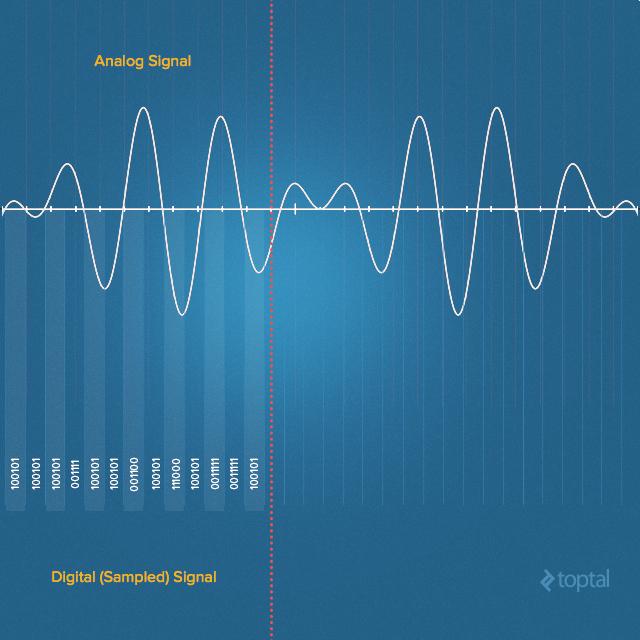
Analog (continuous) and digital (discrete) signals
Thanks to the Kotelnikov theorem, we know what sampling frequency is needed in order to accurately represent a continuous signal limited by a certain frequency. In particular, in order to capture the entire frequency spectrum of sounds accessible to human hearing, we must use a sampling frequency twice as high as the upper limit of frequencies heard by humans.
Namely, a person can hear sounds in the range of approximately from 20 Hz to 20,000 Hz. As a result, sound is most often recorded at a sampling rate of 44,100 Hz. It is this sampling rate that is used in compact discs . It is also most often used for audio coding in the MPEG-1 standard group ( VCD , SVCD , MP3 ).
The widespread use of the sampling rate of 44,100 Hz, we are obliged, mainly, to Sony. At one time, audio tracks encoded in this way were conveniently combined with video in PAL (25 frames per second) and NTSC (30 frames per second) standards , and working with them using existing equipment. It is also very important that this frequency is sufficient for high-quality sound transmission in the range up to 20,000 Hz. Digital audio equipment using this sampling rate is quite consistent in quality with the analog equipment of those times when digital audio standards were becoming established. As a result, choosing the sampling rate for sound when recording, you will most likely stop at 44,100 Hz.
Recording a sampled audio signal is a fairly simple task. Modern sound cards contain built-in analog-to-digital converters. Therefore, it is enough to choose a programming language, find a suitable library for working with sound, specify the sampling frequency, the number of channels (usually one or two, for monophonic and stereo sound, respectively), select the number of bits in one sample (for example, 16 bits are often used) . Then you need to open the data line from the sound card, just like any input stream opens, and write its contents to the byte array. This is how Java does it:
Now it suffices to read the data from the object of the
In our array recorded a digital representation of the audio signal in the time domain . That is, we have information about how the signal amplitude has changed over time.
In the 19th century, Jean Baptiste Joseph Fourier made an outstanding discovery. It consists in the fact that any signal in the time domain is equivalent to the sum of a certain number (possibly infinite) of simple sinusoidal signals, provided that each sinusoid has a certain frequency, amplitude and phase. The set of sinusoids that form the original signal is called the Fourier series .
In other words, one can imagine practically any signal developed in time simply by specifying a set of frequencies, amplitudes and phases corresponding to each of the sinusoids that form this signal. Such a representation of signals is called a set of frequency intervals . In a sense, information about frequency intervals is something like “fingerprints” or signal signatures deployed in time, giving us a static representation of dynamic data.
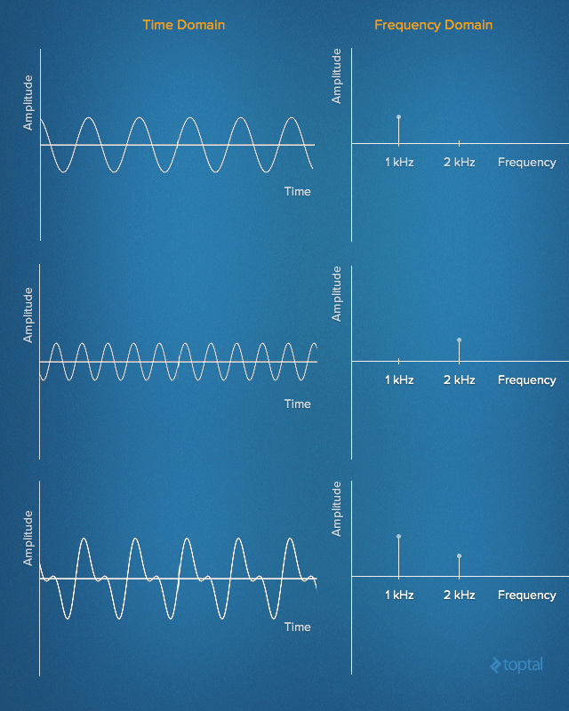
Signals deployed in time and their frequency characteristics
This is what an animated Fourier Series representation for a 1 Hz square wave looks like. It also shows the approximation of the original signal based on a set of sinusoids. In the upper graph, the signal is shown in the amplitude-time domain; in the lower graph, its representation is given in amplitude-frequency form.
Fourier transform in action. Source: Rene Schwarz
Analysis of the frequency characteristics of signals greatly facilitates the solution of many problems. It is very convenient to operate with such characteristics in the field of digital signal processing. They allow studying the spectrum of a signal (its frequency characteristics), determining which frequencies are present in this signal and which are not. After that, you can filter, amplify or weaken some frequencies, or simply recognize the sound of a certain height among the available set of frequencies.
So, you need to find a way to get the frequency characteristics of signals deployed in time. The discrete Fourier transform (DFT, DFT, Discrete Fourier Transform) will help us in this. DFT is a mathematical method of Fourier analysis for discrete signals. It can be used to convert a final set of signal samples taken at equal intervals of time into a list of coefficients of the final combination of complex sinusoids ordered by frequency, taking into account that these sinusoids were disarmed at the same frequency.
One of the most popular numerical algorithms for calculating the DFT is called the Fast Fourier Transform (FFT, FFT, Fast Fourier Transformation). In fact, the FFT is represented by a whole set of algorithms. Among them, the most commonly used variants of the Cooley-Tukey algorithm (Cooley-Tukey). The basis of this algorithm is the principle of "divide and conquer." During calculations, the recursive decomposition of the original DFT into small parts is used. Direct computation of the DFT for some data set n requires O (n 2 ) operations, and the use of the Cooley-Tukey algorithm allows solving the same problem in O (n log n) operations.
It is easy to find a suitable library that implements the FFT algorithm. Here are a few such libraries for different languages:
Here is an example of a function for calculating an FFT written in Java. At its entrance serves complex numbers. In order to understand the relationship between complex numbers and trigonometric functions, it is useful to read about the Euler formula .
Here is an example of a signal before and after FFT analysis.
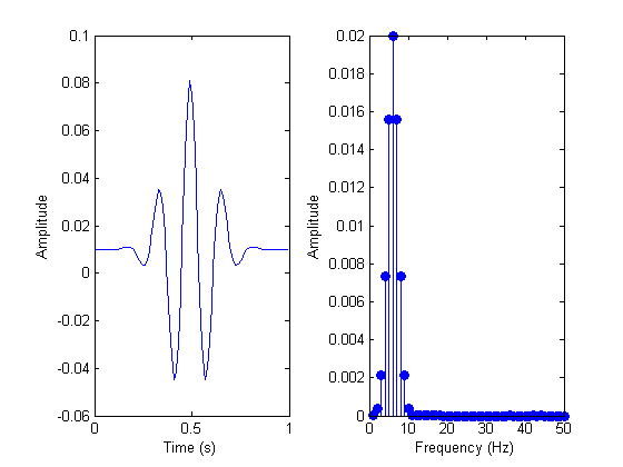
Signal before and after FFT analysis
One of the unpleasant side effects of FFT is that after analyzing, we lose time information. (Although, theoretically, this can be avoided, but in practice this will require enormous computational power.) For example, for a three-minute song we can see sound frequencies and their amplitudes, but we don’t know exactly where these frequencies are in the work. And this is the most important characteristic that makes a piece of music what it is! We need to somehow find out the exact time values when each of the frequencies appears.
That is why we will use something like a sliding window, or a data block, and transform only that part of the signal that gets into this “window”. The size of each block can be determined using different approaches. For example, if we record two-channel sound with a sample size of 16 bits and a sampling frequency of 44100 Hz, one second of such sound will take 176 KB of memory (44100 samples * 2 bytes * 2 channels). If we set the size of the sliding window to 4 KB, then every second we will need to analyze 44 data blocks. This is a fairly high resolution for a detailed analysis of the composition.
Let's go back to programming.
In the internal loop, we put the data from the time domain (sound samples) into complex numbers with an imaginary part equal to 0. In the external loop we go through all the data blocks and run the FFT analysis for each of them.
As soon as we have information about the frequency characteristics of the signal, you can proceed to the formation of a digital signature of a musical work. This is the most important part of the entire music recognition process that Shazam implements. The main difficulty here is to choose from the huge number of frequencies precisely those that are most important. Purely intuitively, we draw attention to frequencies with maximum amplitudes (usually called peaks).
However, in one song the range of “strong” frequencies can vary, say, from the note “to” the counter-instrument (32.70 Hz), to the note “to” the fifth octave (4186.01 Hz). This is a huge interval. Therefore, instead of analyzing the entire frequency range immediately, we can select several smaller intervals. The choice can be made based on the frequencies that are usually inherent in important musical components, and analyzed separately. For example, you can use the intervals that this programmer used to implement his Shazam algorithm. Namely, it is 30 Hz - 40 Hz, 40 Hz - 80 Hz and 80 Hz - 120 Hz for low sounds (this includes, for example, a bass guitar). For medium and higher sounds, frequencies of 120 Hz - 180 Hz and 180 Hz - 300 Hz are used (this includes vocals and most other instruments).
Now that we have decided on intervals, you can simply find the frequencies with the highest levels in them. This information and form the signature for a specific block of data being analyzed, and it, in turn, is part of the signature of the entire song.
Note that we must take into account the fact that the recording was not made in ideal conditions (that is, not in a soundproof room). As a result, it is necessary to provide for the presence of extraneous noise in the recording and possible distortion of the recorded sound, depending on the characteristics of the room. This issue should be approached very seriously, in real systems it is necessary to implement the setting of the analysis of possible distortions and extraneous sounds (fuzz factor) depending on the conditions in which the recording is carried out.
To simplify the search for musical compositions, their signatures are used as keys in a hash table. The keys correspond to the time values when the set of frequencies for which the signature was found appeared in the work, and the identifier of the work itself (the name of the song and the name of the artist, for example). Here is a variant of how such records may look in the database.
If we process a certain library of music records in this way, it will be possible to build a database with full signatures of each piece.
In order to find out what song is playing now in a restaurant, you need to record the sound using the phone and drive it through the above-described process of calculating signatures. You can then start a search for the calculated hash tags in the database.
But not everything is so simple. The fact is that many fragments of different works of hash tags are the same. For example, it may turn out that some fragment of song A sounds just like a certain section of song E. And there is nothing surprising. Musicians and composers constantly “borrow” successful musical figures from each other.
Whenever a matching hash tag is found, the number of possible matches decreases, but it is highly likely that only this information will not allow us to narrow the search range so much as to stop on the only correct song. Therefore, in the music recognition algorithm, we need to check something else. Namely - we are talking about time stamps.
The fragment of a song recorded in a restaurant may be from any of its places, so we simply cannot directly compare the relative time inside the recorded fragment with what is in the database.
However, if several matches are found, you can analyze the relative timing of matches, and thus increase the accuracy of the search.
For example, if you look at the table above, you can find that the hash tag 30 51 99 121 195 applies to song A and song E. If a second later we check the hash tag 34 57 95 111 200, we will find another coinciding with song A, besides, in a similar case we will know that both hash tags and their distribution in time coincide.
Let i1 and i2 be the time stamps in the recorded song, j1 and j2 the time stamps in the song from the database. We can say that there are two coincidences, taking into account the coincidence of the time difference, if the following condition is met:
This makes it possible not to care about exactly what part of the song the recording has: the beginning, the middle, or the very end.
And, finally, it is unlikely that each processed fragment of a song recorded in the “wild” conditions will coincide with a similar fragment from a database built on the basis of studio recordings. Record, on the basis of which we want to find the name of the work, will include a lot of noise, which will lead to some discrepancies in the comparison. Therefore, instead of trying to exclude everything from the list of matches, except for the only correct composition, at the end of the database mapping procedure, we will sort the records in which there were matches. We will sort in descending order. The more matches there are, the more likely it is that we find the right composition. Accordingly, she will be at the top of the list.
Here is an overview of the entire procedure for recognizing music. Walk on it from start to finish.
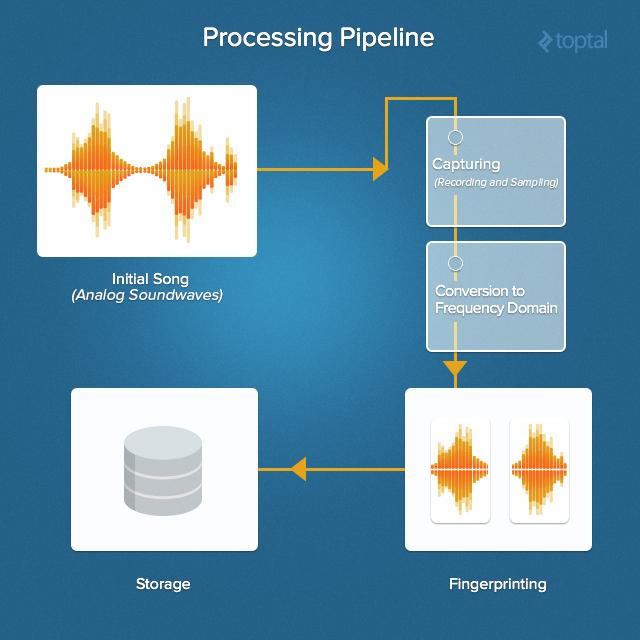
Music Recognition Review
It all starts with the original sound. Then it is captured, find the frequency characteristics, compute hash tags and compare them with those stored in the music database.
In such systems, databases can be huge, so it is important to use solutions that can be scaled. There is no particular need for database table links, the data model is very simple, so some kind of NoSQL database is quite suitable here.
Programs like the one we talked about here are suitable for finding similar places in musical works. Now that you understand how Shazam works, you can see that the music recognition algorithms are applicable not only as “reminders” of the names of forgotten songs from the past that are heard on the radio in a taxi.
For example, you can use them to look for musical plagiarism, or use them to find performers who inspired some pioneers in blues, jazz, rock music, pop music, and in any other genre.
Perhaps a good experiment will be filling the database with classics — the writings of Bach, Beethoven, Vivaldi, Wagner, Chopin, and Mozart and searching for similar things in their works. It is quite possible to find out that even Bob Dylan, Elvis Presley and Robert Johnson were not averse to borrow anything from others!
But can we blame them for it? I'm sure not. After all, music is just a sound wave that a person hears, remembers and repeats in his head. There it develops, changes - until it is recorded in the studio and released into the wild, where it can quite inspire another genius from music.
You have a smartphone in your pocket, which has a program for recognizing music. This program is your savior. In order to find out the name of the song, you will not have to walk from corner to corner in an attempt to extract the cherished line from your own memory. And after all not the fact that it will turn out. The program, if you let it “listen” to the music, immediately reports the name of the composition. After that, you can listen to the sweet heart sounds again and again. Until they become one with you, or - until you get tired of all this.
Mobile technologies and incredible progress in the field of sound processing give algorithm developers the ability to create music recognition applications. One of the most popular solutions of this kind is called Shazam . If you give it 20 seconds of sound, no matter whether it is a piece of an intro, chorus or part of the main motive, Shazam will create a signature code, check the database and use its own music recognition algorithm to give the name of the piece.
')
How does all this work?
The description of the basic Shazam algorithm in 2003 was published by its creator, Avery Li-Chung Wang (Avery Li-Chung Wang). In this article, we will examine in detail the basics of the Shazam music recognition algorithm.
From analog to digital: discretization
What is sound, really? Maybe it is some mysterious bodiless substance that penetrates our ears and allows us to hear?
Of course, everything is not so mysterious. It has long been known that sound is mechanical vibrations that propagate in solid, liquid and gaseous media in the form of elastic waves. When the wave reaches the ear, in particular - the eardrum, the auditory ossicles are set in motion, which transmit vibrations further to the hair cells located in the inner ear. As a result, mechanical vibrations are converted into electrical impulses that are transmitted through the auditory nerves to the brain.
Devices for recording sound imitate the above process quite accurately, converting the pressure of a sound wave into an electrical signal. A sound wave in air is a continuous signal, represented by areas of compression and rarefaction. The microphone, the first electronic component with which the sound signal is encountered, converts it into an electrical signal, which is still continuous. Such signals in the digital world are not particularly useful, therefore, before storage and processing in digital systems, they need to be converted to discrete form. This is done by sampling the values representing the amplitude values of the signal.
In the process of such a conversion, the analog signal is quantized . It does not do without a small number of errors. Thus, we are not dealing with a single-step conversion; the analog-to-digital converter performs many operations on the conversion of very small parts of an analog signal into a digital one. This process is called sampling or sampling.
Analog (continuous) and digital (discrete) signals
Thanks to the Kotelnikov theorem, we know what sampling frequency is needed in order to accurately represent a continuous signal limited by a certain frequency. In particular, in order to capture the entire frequency spectrum of sounds accessible to human hearing, we must use a sampling frequency twice as high as the upper limit of frequencies heard by humans.
Namely, a person can hear sounds in the range of approximately from 20 Hz to 20,000 Hz. As a result, sound is most often recorded at a sampling rate of 44,100 Hz. It is this sampling rate that is used in compact discs . It is also most often used for audio coding in the MPEG-1 standard group ( VCD , SVCD , MP3 ).
The widespread use of the sampling rate of 44,100 Hz, we are obliged, mainly, to Sony. At one time, audio tracks encoded in this way were conveniently combined with video in PAL (25 frames per second) and NTSC (30 frames per second) standards , and working with them using existing equipment. It is also very important that this frequency is sufficient for high-quality sound transmission in the range up to 20,000 Hz. Digital audio equipment using this sampling rate is quite consistent in quality with the analog equipment of those times when digital audio standards were becoming established. As a result, choosing the sampling rate for sound when recording, you will most likely stop at 44,100 Hz.
Record: capture sound
Recording a sampled audio signal is a fairly simple task. Modern sound cards contain built-in analog-to-digital converters. Therefore, it is enough to choose a programming language, find a suitable library for working with sound, specify the sampling frequency, the number of channels (usually one or two, for monophonic and stereo sound, respectively), select the number of bits in one sample (for example, 16 bits are often used) . Then you need to open the data line from the sound card, just like any input stream opens, and write its contents to the byte array. This is how Java does it:
private AudioFormat getFormat() { float sampleRate = 44100; int sampleSizeInBits = 16; int channels = 1; // boolean signed = true; // , boolean bigEndian = true; // , (big-endian) (little-endian) return new AudioFormat(sampleRate, sampleSizeInBits, channels, signed, bigEndian); } final AudioFormat format = getFormat(); // AudioFormat DataLine.Info info = new DataLine.Info(TargetDataLine.class, format); final TargetDataLine line = (TargetDataLine) AudioSystem.getLine(info); line.open(format); line.start(); Now it suffices to read the data from the object of the
TargetDataLine class. In the example, the flag is running , it is a global variable that can be accessed from another thread. For example, such a variable will allow us to stop capturing sound from the user interface stream using the Stop button. OutputStream out = new ByteArrayOutputStream(); running = true; try { while (running) { int count = line.read(buffer, 0, buffer.length); if (count > 0) { out.write(buffer, 0, count); } } out.close(); } catch (IOException e) { System.err.println("I/O problems: " + e); System.exit(-1); } Time and frequency domains
In our array recorded a digital representation of the audio signal in the time domain . That is, we have information about how the signal amplitude has changed over time.
In the 19th century, Jean Baptiste Joseph Fourier made an outstanding discovery. It consists in the fact that any signal in the time domain is equivalent to the sum of a certain number (possibly infinite) of simple sinusoidal signals, provided that each sinusoid has a certain frequency, amplitude and phase. The set of sinusoids that form the original signal is called the Fourier series .
In other words, one can imagine practically any signal developed in time simply by specifying a set of frequencies, amplitudes and phases corresponding to each of the sinusoids that form this signal. Such a representation of signals is called a set of frequency intervals . In a sense, information about frequency intervals is something like “fingerprints” or signal signatures deployed in time, giving us a static representation of dynamic data.
Signals deployed in time and their frequency characteristics
This is what an animated Fourier Series representation for a 1 Hz square wave looks like. It also shows the approximation of the original signal based on a set of sinusoids. In the upper graph, the signal is shown in the amplitude-time domain; in the lower graph, its representation is given in amplitude-frequency form.
Fourier transform in action. Source: Rene Schwarz
Analysis of the frequency characteristics of signals greatly facilitates the solution of many problems. It is very convenient to operate with such characteristics in the field of digital signal processing. They allow studying the spectrum of a signal (its frequency characteristics), determining which frequencies are present in this signal and which are not. After that, you can filter, amplify or weaken some frequencies, or simply recognize the sound of a certain height among the available set of frequencies.
Discrete Fourier Transform
So, you need to find a way to get the frequency characteristics of signals deployed in time. The discrete Fourier transform (DFT, DFT, Discrete Fourier Transform) will help us in this. DFT is a mathematical method of Fourier analysis for discrete signals. It can be used to convert a final set of signal samples taken at equal intervals of time into a list of coefficients of the final combination of complex sinusoids ordered by frequency, taking into account that these sinusoids were disarmed at the same frequency.
One of the most popular numerical algorithms for calculating the DFT is called the Fast Fourier Transform (FFT, FFT, Fast Fourier Transformation). In fact, the FFT is represented by a whole set of algorithms. Among them, the most commonly used variants of the Cooley-Tukey algorithm (Cooley-Tukey). The basis of this algorithm is the principle of "divide and conquer." During calculations, the recursive decomposition of the original DFT into small parts is used. Direct computation of the DFT for some data set n requires O (n 2 ) operations, and the use of the Cooley-Tukey algorithm allows solving the same problem in O (n log n) operations.
It is easy to find a suitable library that implements the FFT algorithm. Here are a few such libraries for different languages:
- C - FFTW
- C ++ - EigenFFT
- Java - JTransform
- Python - NumPy
- Ruby - Ruby-FFTW3 (interface to FFTW)
Here is an example of a function for calculating an FFT written in Java. At its entrance serves complex numbers. In order to understand the relationship between complex numbers and trigonometric functions, it is useful to read about the Euler formula .
public static Complex[] fft(Complex[] x) { int N = x.length; // fft Complex[] even = new Complex[N / 2]; for (int k = 0; k < N / 2; k++) { even[k] = x[2 * k]; } Complex[] q = fft(even); // fft Complex[] odd = even; // for (int k = 0; k < N / 2; k++) { odd[k] = x[2 * k + 1]; } Complex[] r = fft(odd); // Complex[] y = new Complex[N]; for (int k = 0; k < N / 2; k++) { double kth = -2 * k * Math.PI / N; Complex wk = new Complex(Math.cos(kth), Math.sin(kth)); y[k] = q[k].plus(wk.times(r[k])); y[k + N / 2] = q[k].minus(wk.times(r[k])); } return y; } Here is an example of a signal before and after FFT analysis.
Signal before and after FFT analysis
Music Recognition: Song Signatures
One of the unpleasant side effects of FFT is that after analyzing, we lose time information. (Although, theoretically, this can be avoided, but in practice this will require enormous computational power.) For example, for a three-minute song we can see sound frequencies and their amplitudes, but we don’t know exactly where these frequencies are in the work. And this is the most important characteristic that makes a piece of music what it is! We need to somehow find out the exact time values when each of the frequencies appears.
That is why we will use something like a sliding window, or a data block, and transform only that part of the signal that gets into this “window”. The size of each block can be determined using different approaches. For example, if we record two-channel sound with a sample size of 16 bits and a sampling frequency of 44100 Hz, one second of such sound will take 176 KB of memory (44100 samples * 2 bytes * 2 channels). If we set the size of the sliding window to 4 KB, then every second we will need to analyze 44 data blocks. This is a fairly high resolution for a detailed analysis of the composition.
Let's go back to programming.
byte audio [] = out.toByteArray() int totalSize = audio.length int sampledChunkSize = totalSize/chunkSize; Complex[][] result = ComplexMatrix[sampledChunkSize][]; for(int j = 0;i < sampledChunkSize; j++) { Complex[chunkSize] complexArray; for(int i = 0; i < chunkSize; i++) { complexArray[i] = Complex(audio[(j*chunkSize)+i], 0); } result[j] = FFT.fft(complexArray); } In the internal loop, we put the data from the time domain (sound samples) into complex numbers with an imaginary part equal to 0. In the external loop we go through all the data blocks and run the FFT analysis for each of them.
As soon as we have information about the frequency characteristics of the signal, you can proceed to the formation of a digital signature of a musical work. This is the most important part of the entire music recognition process that Shazam implements. The main difficulty here is to choose from the huge number of frequencies precisely those that are most important. Purely intuitively, we draw attention to frequencies with maximum amplitudes (usually called peaks).
However, in one song the range of “strong” frequencies can vary, say, from the note “to” the counter-instrument (32.70 Hz), to the note “to” the fifth octave (4186.01 Hz). This is a huge interval. Therefore, instead of analyzing the entire frequency range immediately, we can select several smaller intervals. The choice can be made based on the frequencies that are usually inherent in important musical components, and analyzed separately. For example, you can use the intervals that this programmer used to implement his Shazam algorithm. Namely, it is 30 Hz - 40 Hz, 40 Hz - 80 Hz and 80 Hz - 120 Hz for low sounds (this includes, for example, a bass guitar). For medium and higher sounds, frequencies of 120 Hz - 180 Hz and 180 Hz - 300 Hz are used (this includes vocals and most other instruments).
Now that we have decided on intervals, you can simply find the frequencies with the highest levels in them. This information and form the signature for a specific block of data being analyzed, and it, in turn, is part of the signature of the entire song.
public final int[] RANGE = new int[] { 40, 80, 120, 180, 300 }; // , public int getIndex(int freq) { int i = 0; while (RANGE[i] < freq) i++; return i; } // – , for (int t = 0; t < result.length; t++) { for (int freq = 40; freq < 300 ; freq++) { // : double mag = Math.log(results[t][freq].abs() + 1); // , : int index = getIndex(freq); // : if (mag > highscores[t][index]) { points[t][index] = freq; } } // - long h = hash(points[t][0], points[t][1], points[t][2], points[t][3]); } private static final int FUZ_FACTOR = 2; private long hash(long p1, long p2, long p3, long p4) { return (p4 - (p4 % FUZ_FACTOR)) * 100000000 + (p3 - (p3 % FUZ_FACTOR)) * 100000 + (p2 - (p2 % FUZ_FACTOR)) * 100 + (p1 - (p1 % FUZ_FACTOR)); } Note that we must take into account the fact that the recording was not made in ideal conditions (that is, not in a soundproof room). As a result, it is necessary to provide for the presence of extraneous noise in the recording and possible distortion of the recorded sound, depending on the characteristics of the room. This issue should be approached very seriously, in real systems it is necessary to implement the setting of the analysis of possible distortions and extraneous sounds (fuzz factor) depending on the conditions in which the recording is carried out.
To simplify the search for musical compositions, their signatures are used as keys in a hash table. The keys correspond to the time values when the set of frequencies for which the signature was found appeared in the work, and the identifier of the work itself (the name of the song and the name of the artist, for example). Here is a variant of how such records may look in the database.
| Hash tag | Time in seconds | Song |
| 30 51 99 121 195 | 53.52 | Song A Artist A |
| 33 56 92 151 185 | 12.32 | Song B Artist B |
| 39 26 89 141 251 | 15.34 | Song C Artist C |
| 32 67,100 128,270 | 78.43 | Song D Artist D |
| 30 51 99 121 195 | 10.89 | Song E of artist E |
| 34 57 95 111 200 | 54.52 | Song A Artist A |
| 34 41 93 161 202 | 11.89 | Song E of artist E |
If we process a certain library of music records in this way, it will be possible to build a database with full signatures of each piece.
Match Search
In order to find out what song is playing now in a restaurant, you need to record the sound using the phone and drive it through the above-described process of calculating signatures. You can then start a search for the calculated hash tags in the database.
But not everything is so simple. The fact is that many fragments of different works of hash tags are the same. For example, it may turn out that some fragment of song A sounds just like a certain section of song E. And there is nothing surprising. Musicians and composers constantly “borrow” successful musical figures from each other.
Whenever a matching hash tag is found, the number of possible matches decreases, but it is highly likely that only this information will not allow us to narrow the search range so much as to stop on the only correct song. Therefore, in the music recognition algorithm, we need to check something else. Namely - we are talking about time stamps.
The fragment of a song recorded in a restaurant may be from any of its places, so we simply cannot directly compare the relative time inside the recorded fragment with what is in the database.
However, if several matches are found, you can analyze the relative timing of matches, and thus increase the accuracy of the search.
For example, if you look at the table above, you can find that the hash tag 30 51 99 121 195 applies to song A and song E. If a second later we check the hash tag 34 57 95 111 200, we will find another coinciding with song A, besides, in a similar case we will know that both hash tags and their distribution in time coincide.
// , private class DataPoint { private int time; private int songId; public DataPoint(int songId, int time) { this.songId = songId; this.time = time; } public int getTime() { return time; } public int getSongId() { return songId; } } Let i1 and i2 be the time stamps in the recorded song, j1 and j2 the time stamps in the song from the database. We can say that there are two coincidences, taking into account the coincidence of the time difference, if the following condition is met:
RecordedHash(i1) = SongInDBHash(j1) AND RecordedHash(i2) = SongInDBHash(j2) AND abs(i1 - i2) = abs (j1 - j2) This makes it possible not to care about exactly what part of the song the recording has: the beginning, the middle, or the very end.
And, finally, it is unlikely that each processed fragment of a song recorded in the “wild” conditions will coincide with a similar fragment from a database built on the basis of studio recordings. Record, on the basis of which we want to find the name of the work, will include a lot of noise, which will lead to some discrepancies in the comparison. Therefore, instead of trying to exclude everything from the list of matches, except for the only correct composition, at the end of the database mapping procedure, we will sort the records in which there were matches. We will sort in descending order. The more matches there are, the more likely it is that we find the right composition. Accordingly, she will be at the top of the list.
Music Recognition Review
Here is an overview of the entire procedure for recognizing music. Walk on it from start to finish.
Music Recognition Review
It all starts with the original sound. Then it is captured, find the frequency characteristics, compute hash tags and compare them with those stored in the music database.
In such systems, databases can be huge, so it is important to use solutions that can be scaled. There is no particular need for database table links, the data model is very simple, so some kind of NoSQL database is quite suitable here.
Shazam!
Programs like the one we talked about here are suitable for finding similar places in musical works. Now that you understand how Shazam works, you can see that the music recognition algorithms are applicable not only as “reminders” of the names of forgotten songs from the past that are heard on the radio in a taxi.
For example, you can use them to look for musical plagiarism, or use them to find performers who inspired some pioneers in blues, jazz, rock music, pop music, and in any other genre.
Perhaps a good experiment will be filling the database with classics — the writings of Bach, Beethoven, Vivaldi, Wagner, Chopin, and Mozart and searching for similar things in their works. It is quite possible to find out that even Bob Dylan, Elvis Presley and Robert Johnson were not averse to borrow anything from others!
But can we blame them for it? I'm sure not. After all, music is just a sound wave that a person hears, remembers and repeats in his head. There it develops, changes - until it is recorded in the studio and released into the wild, where it can quite inspire another genius from music.
Oh, and come to work with us? :)wunderfund.io is a young foundation that deals with high-frequency algorithmic trading . High-frequency trading is a continuous competition of the best programmers and mathematicians of the whole world. By joining us, you will become part of this fascinating fight.
We offer interesting and challenging data analysis and low latency tasks for enthusiastic researchers and programmers.
Flexible schedule and no bureaucracy, decisions are quickly made and implemented.
Join our team: wunderfund.io
Source: https://habr.com/ru/post/275043/
All Articles