Concurrent programming with CUDA. Part 2: GPU hardware and parallel communication patterns

Content

Parallel communication patterns

• run along the stream to each output element, where each stream will average the values ​​of 3 neighboring input elements - gather ;
• or run downstream to each input element, where each stream will add 1/3 of the value of its input element to the value of the corresponding output element - scatter .

1. All data needed for one stream is grouped in memory (in the case of a one-dimensional array, a solid “piece” of memory, in the 2D case, several pieces of memory that are at the same distance from each other).
2. The value of some input element is read several times from neighboring streams (the specific number of readings depends on the selected mask) - it becomes possible to "reuse" the data provided to us by CUDA - this will be discussed later in the article.

GPU hardware

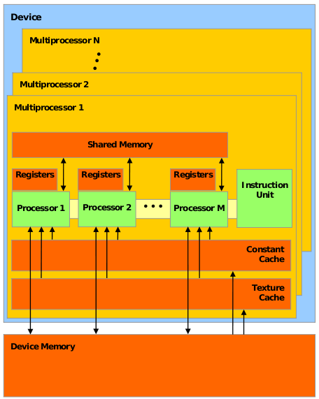
• A CUDA-compatible GPU consists of several (usually dozens) streaming multiprocessors (streaming multiprocessors), followed by SM .
• Each SM , in turn, consists of several dozen simple / streaming processors (SP) (regular / stream processors), or to put it more precisely, CUDA cores ( CUDA cores ). These guys are more like the usual CPU - they have their own registers, cache, etc. Each SM also has its own shared memory (shared memory) —a kind of additional cache that is accessible to all SPs, and can be used both as a cache for frequently used data and for “communication” between threads of a single CUDA block.
• The GPU also has its own memory, called device memory , which is common to all CUDA streams - the cudaMalloc and cudaMemcpy functions work with it (it is also the size used by schoolchildren and GPU manufacturers to compare with its size) .

Compliance with CUDA model and GPU hardware. CUDA Warranties

• Each block will be completely executed on the SM allocated to it.
• The distribution of blocks on the SM is engaged in the GPU, not the programmer.
• All streams of block X will be divided into groups, called warps (usually say so - warps), and executed on the SM . The size of these groups depends on the GPU model, for example, for models with the Fermi microarchitecture, it is equal to 32. All threads from the same warp are executed at the same time, occupying a certain part of the SM resources. And they either perform the same instruction (but on different data), or idle.

• All threads in a particular block will be executed on any one SM .
• All threads of a specific kernel will be executed before the next kernel starts.

• Any block X will be executed before / after / simultaneously with some block Y.
• Some block X will be executed on some particular SM Z.

Synchronization

• A barrier is a point in the code of the kernel, upon reaching which a thread can “pass” further only if all the threads from its block have reached this point. Once again: the barrier allows you to synchronize only the threads of one block , and not all the threads in principle! The restriction is quite natural, because the number of blocks set by the programmer can significantly exceed the number of available SMs .
• Atomic operations are similar to atomic operations of the CPU, the full list of available operations can be found here .
• __threadfence is not exactly a synchronization primitive: when this instruction is reached, a thread can continue execution only after all its memory manipulations become visible to other threads - in effect, it forces the thread to flush the cache.

Basic principles for the effective use of CUDA

• The principle of increasing the ratio (useful time) / (time of memory operations) - was discussed in the previous article. The fraction value can be increased in two ways - to increase the numerator, to reduce the denominator: that is, you need to either do more work, or spend less time on memory operations. In addition to the obvious solution - to reduce the number of memory accesses as far as possible, the following principles of efficient work with memory are used:
  
  
  • Moving frequently used data to faster memory: local stream memory > shared block memory >> shared device memory >> host memory. Thus, if several streams in the same block use the same data, it is most likely that it makes sense to move them to the common memory of the block.
  • Sequential memory access: since the streams in the blocks are actually running in warp groups, provided that the streams in the same warp work with data located in memory sequentially, CUDA can read one large chunk of memory as one instruction. Otherwise, if the streams in the warp will access the data scattered in the memory, the number of memory accesses will increase.
  
  
  
• Reducing divergence of flows: a feature of the work of CUDA is that the threads in the same warp always either execute the same instruction or idle. Thus, if in the kernel code there is code of the form
  
  

  if (threadIdx.x % 2 == 0) { ... } ... 

  
  
  , then half of the warp threads (those with an odd index) will wait for the other half to execute the code inside the if-a. Therefore, you should avoid such situations.

Writing a second program on CUDA

 #include <chrono> #include <iostream> #include <cstring> #include <string> #include <opencv2/core/core.hpp> #include <opencv2/highgui/highgui.hpp> #include <opencv2/opencv.hpp> #include <vector_types.h> #include "openMP.hpp" #include "CUDA_wrappers.hpp" #include "common/image_helpers.hpp" void prepareFilter(float **filter, int *filterWidth, float *filterSigma) { static const int blurFilterWidth = 9; static const float blurFilterSigma = 2.; *filter = new float[blurFilterWidth * blurFilterWidth]; *filterWidth = blurFilterWidth; *filterSigma = blurFilterSigma; float filterSum = 0.f; const int halfWidth = blurFilterWidth/2; for (int r = -halfWidth; r <= halfWidth; ++r) { for (int c = -halfWidth; c <= halfWidth; ++c) { float filterValue = expf( -(float)(c * c + r * r) / (2.f * blurFilterSigma * blurFilterSigma)); (*filter)[(r + halfWidth) * blurFilterWidth + c + halfWidth] = filterValue; filterSum += filterValue; } } float normalizationFactor = 1.f / filterSum; for (int r = -halfWidth; r <= halfWidth; ++r) { for (int c = -halfWidth; c <= halfWidth; ++c) { (*filter)[(r + halfWidth) * blurFilterWidth + c + halfWidth] *= normalizationFactor; } } } void freeFilter(float *filter) { delete[] filter; } int main( int argc, char** argv ) { using namespace cv; using namespace std; using namespace std::chrono; if( argc != 2) { cout <<" Usage: blur_image imagefile" << endl; return -1; } Mat image, blurredImage, referenceBlurredImage; uchar4 *imageArray, *blurredImageArray; prepareImagePointers(argv[1], image, &imageArray, blurredImage, &blurredImageArray, CV_8UC4); int numRows = image.rows, numCols = image.cols; float *filter, filterSigma; int filterWidth; prepareFilter(&filter, &filterWidth, &filterSigma); cv::Size filterSize(filterWidth, filterWidth); auto start = system_clock::now(); cv::GaussianBlur(image, referenceBlurredImage, filterSize, filterSigma, filterSigma, BORDER_REPLICATE); auto duration = duration_cast<milliseconds>(system_clock::now() - start); cout<<"OpenCV time (ms):" << duration.count() << endl; start = system_clock::now(); BlurImageOpenMP(imageArray, blurredImageArray, numRows, numCols, filter, filterWidth); duration = duration_cast<milliseconds>(system_clock::now() - start); cout<<"OpenMP time (ms):" << duration.count() << endl; cout<<"OpenMP similarity:" << getEuclidianSimilarity(referenceBlurredImage, blurredImage) << endl; for (int i=0; i<4; ++i) { memset(blurredImageArray, 0, sizeof(uchar4)*numRows*numCols); start = system_clock::now(); BlurImageCUDA(imageArray, blurredImageArray, numRows, numCols, filter, filterWidth); duration = duration_cast<milliseconds>(system_clock::now() - start); cout<<"CUDA time full (ms):" << duration.count() << endl; cout<<"CUDA similarity:" << getEuclidianSimilarity(referenceBlurredImage, blurredImage) << endl; } freeFilter(filter); return 0; } 

1. We read the image file, prepare pointers to the original image and the resulting blurred image. The prepareImagePointers function remains the same; if necessary, you can view its source code on bitbucket.
2. Prepare a Gaussian filter - that is, a set of our scales. We also remember the used filter parameters in order to transfer them to OpenCV and get a sample of the blurred image to verify the correctness of our algorithms.
3. Call the Gauss blur function from OpenCV, save the resulting sample, measure the time spent.
4. Call the Gauss blur function written using OpenMP, measure the time spent, check the result obtained with the sample. The image similarity calculation function of getEuclidianSimilarity is as follows:
   
   
   getEuclidianSimilarity

    double getEuclidianSimilarity(const cv::Mat& a, const cv::Mat& b) { double errorL2 = cv::norm(a, b, cv::NORM_L2); double similarity = errorL2 / (double) (a.rows * a.cols); return similarity; } 

   
   
   
   
   
   In fact, it finds the average sum of squares of differences in the values ​​of all channels of all pixels of two images.
5. Call the CUDA-version of the blur according to Gauss 4 times, each time measuring the time spent and checking the obtained result with the sample. Why call 4 times? The fact is that with the very first call, some time will be spent on initialization - therefore, it is better to run several times and measure the time spent on subsequent calls.

 #include <stdio.h> #include <omp.h> #include <vector_types.h> #include <vector_functions.h> void BlurImageOpenMP(const uchar4 * const imageArray, uchar4 * const blurredImageArray, const long numRows, const long numCols, const float * const filter, const size_t filterWidth) { using namespace std; const long halfWidth = filterWidth/2; #pragma omp parallel for collapse(2) for (long row = 0; row < numRows; ++row) { for (long col = 0; col < numCols; ++col) { float resR=0.0f, resG=0.0f, resB=0.0f; for (long filterRow = -halfWidth; filterRow <= halfWidth; ++filterRow) { for (long filterCol = -halfWidth; filterCol <= halfWidth; ++filterCol) { //Find the global image position for this filter position //clamp to boundary of the image const long imageRow = min(max(row + filterRow, static_cast<long>(0)), numRows - 1); const long imageCol = min(max(col + filterCol, static_cast<long>(0)), numCols - 1); const uchar4 imagePixel = imageArray[imageRow*numCols+imageCol]; const float filterValue = filter[(filterRow+halfWidth)*filterWidth+filterCol+halfWidth]; resR += imagePixel.x*filterValue; resG += imagePixel.y*filterValue; resB += imagePixel.z*filterValue; } } blurredImageArray[row*numCols+col] = make_uchar4(resR, resG, resB, 255); } } } 

 #include <iostream> #include <cuda.h> #include "CUDA_wrappers.hpp" #include "common/CUDA_common.hpp" __global__ void gaussian_blur(const uchar4* const d_image, uchar4* const d_blurredImage, const int numRows, const int numCols, const float * const d_filter, const int filterWidth) { const int row = blockIdx.y*blockDim.y+threadIdx.y; const int col = blockIdx.x*blockDim.x+threadIdx.x; if (col >= numCols || row >= numRows) return; const int halfWidth = filterWidth/2; extern __shared__ float shared_filter[]; if (threadIdx.y < filterWidth && threadIdx.x < filterWidth) { const int filterOff = threadIdx.y*filterWidth+threadIdx.x; shared_filter[filterOff] = d_filter[filterOff]; } __syncthreads(); float resR=0.0f, resG=0.0f, resB=0.0f; for (int filterRow = -halfWidth; filterRow <= halfWidth; ++filterRow) { for (int filterCol = -halfWidth; filterCol <= halfWidth; ++filterCol) { //Find the global image position for this filter position //clamp to boundary of the image const int imageRow = min(max(row + filterRow, 0), numRows - 1); const int imageCol = min(max(col + filterCol, 0), numCols - 1); const uchar4 imagePixel = d_image[imageRow*numCols+imageCol]; const float filterValue = shared_filter[(filterRow+halfWidth)*filterWidth+filterCol+halfWidth]; resR += imagePixel.x * filterValue; resG += imagePixel.y * filterValue; resB += imagePixel.z * filterValue; } } d_blurredImage[row*numCols+col] = make_uchar4(resR, resG, resB, 255); } void BlurImageCUDA(const uchar4 * const h_image, uchar4 * const h_blurredImage, const size_t numRows, const size_t numCols, const float * const h_filter, const size_t filterWidth) { uchar4 *d_image, *d_blurredImage; cudaSetDevice(0); checkCudaErrors(cudaGetLastError()); const size_t numPixels = numRows * numCols; const size_t imageSize = sizeof(uchar4) * numPixels; //allocate memory on the device for both input and output checkCudaErrors(cudaMalloc(&d_image, imageSize)); checkCudaErrors(cudaMalloc(&d_blurredImage, imageSize)); //copy input array to the GPU checkCudaErrors(cudaMemcpy(d_image, h_image, imageSize, cudaMemcpyHostToDevice)); float *d_filter; const size_t filterSize = sizeof(float) * filterWidth * filterWidth; checkCudaErrors(cudaMalloc(&d_filter, filterSize)); checkCudaErrors(cudaMemcpy(d_filter, h_filter, filterSize, cudaMemcpyHostToDevice)); dim3 blockSize; dim3 gridSize; int threadNum; cudaEvent_t start, stop; cudaEventCreate(&start); cudaEventCreate(&stop); threadNum = 32; blockSize = dim3(threadNum, threadNum, 1); gridSize = dim3(numCols/threadNum+1, numRows/threadNum+1, 1); cudaEventRecord(start); gaussian_blur<<<gridSize, blockSize, filterSize>>>(d_image, d_blurredImage, numRows, numCols, d_filter, filterWidth); cudaEventRecord(stop); cudaEventSynchronize(stop); cudaDeviceSynchronize(); checkCudaErrors(cudaGetLastError()); float milliseconds = 0; cudaEventElapsedTime(&milliseconds, start, stop); std::cout << "CUDA time kernel (ms): " << milliseconds << std::endl; checkCudaErrors(cudaMemcpy(h_blurredImage, d_blurredImage, sizeof(uchar4) * numPixels, cudaMemcpyDeviceToHost)); checkCudaErrors(cudaFree(d_filter)); checkCudaErrors(cudaFree(d_image)); checkCudaErrors(cudaFree(d_blurredImage)); } 

1. Allocate memory on the device for the original image, output image, filter. Copy the relevant data from the host memory to the allocated device memory.
2. Call the core. Pay attention to the new, 3rd parameter when you call the kernel: <<< gridSize, blockSize, filterSize >>> - it sets the size of the total memory that is needed for each block. In this task, it was possible to realize the use of shared memory in two ways: either move the filter data to the common memory of the block, or move the “piece” of the image that only this block needs, since it is these data that are needed by several threads of the block at once. However, the second option is somewhat more complicated - you need to take into account that the piece of the input image that is needed for each block is slightly larger than the block itself - because we perform the gather operation, which means each stream calculates the values ​​of one pixel of the output image using several neighboring pixels of the original image:
   
   
   
   Therefore, I stopped at the first option, which means that each block needs exactly sizeof (float) * filterWidth * filterWidth memory to store all filter values. Moving the filter weights from the device’s memory to the block’s common memory is as follows:
   
   
   Hidden text

     extern __shared__ float shared_filter[]; if (threadIdx.y < filterWidth && threadIdx.x < filterWidth) { const int filterOff = threadIdx.y*filterWidth+threadIdx.x; shared_filter[filterOff] = d_filter[filterOff]; } __syncthreads(); 

   
   
   
   
   
   Here __shared__ in the declaration of the filter weights array says that this data should be placed in the shared memory of the block; extern means that the size of the allocated memory will be set at the location of the kernel call; __syncthreads is a barrier that guarantees that all filter weights will be transferred to the common memory of the block before any of the threads of this block continues its execution. Further, all readings of the filter weights are made from the total memory of the block.
3. Copy the output image from the device memory to the host memory, freeing the allocated memory.

 OpenCV time (ms):2 OpenMP time (ms):11 OpenMP similarity:0.00287131 CUDA time kernel (ms): 2.93245 CUDA time full (ms):32 CUDA similarity:0.00287131 CUDA time kernel (ms): 2.93402 CUDA time full (ms):4 CUDA similarity:0.00287131 CUDA time kernel (ms): 2.93267 CUDA time full (ms):4 CUDA similarity:0.00287131 CUDA time kernel (ms): 2.93312 CUDA time full (ms):4 CUDA similarity:0.00287131