Evolutionary Computing: Learning to Walk a Stool

This tutorial is dedicated to evolutionary computing, how they work and how to implement them in their projects and games. After reading the article, you will be able to master the power of evolution to find solutions to problems that you are unable to solve. As an example, this tutorial will show how evolutionary computing can be used to teach a simple creature to walk. If you want to experience the power of evolutionary computing in the browser, check out Genetic Algorithm Walkers .

Part 1. Theory

Introduction

As a programmer, you are probably familiar with the concept of the algorithm. If you have a problem, then you write a clear set of instructions for solving it. But what happens when the task is too complicated, or you do not understand how to solve it? There is a very clear strategy for an optimal sudoku game, but not for face recognition. How to code a solution to a problem, if you have no idea how to solve it?

')

In this case, artificial intelligence is usually used. One of the simplest techniques that can be used to solve this class of problems is evolutionary computation . In short, they are based on the idea of ​​applying Darwinian evolution to a computer program. The goal of evolution is to improve the quality of a bad solution with random mutations until the problem is solved with the necessary accuracy. In this tutorial, we will look at how evolutionary computations can be applied to teach optimal walking strategies. A more complex implementation can be seen in the video below (article: Flexible Muscle-Based Locomotion for Bipedal Creatures ).

Natural artificial selection

There is a possibility that you have heard the Darwinian concept of survival of the fittest . The basic idea is simple: survival is a difficult task, and surviving creatures have a higher chance of reproduction. The environment naturally selects the creatures that are most suited to it, killing those who do not cope with this task. This is often demonstrated on an overly simplistic (and misleading) example of giraffes: a longer neck helped giraffes to reach the upper branches. Over time, giraffes were picked with longer and longer necks. There has never been a direct force “lengthening” the neck of a giraffe: the environment itself gradually selected individuals with longer necks.



The same mechanism can be applied to computer programs. If we have an approximate solution to the problem, then we can randomly change it and check whether it has improved its results. If we continue to repeat this process, then as a result we will always get the best (or the same) solution. Natural selection does not depend on the task, in essence it is controlled by random mutations.

Phenotype and genotype

To understand how calculations can be combined with evolution, we first need to understand the role of evolution in biology. In nature, every creature has a body and a set of behaviors. They are known as its phenotype , that is, how the creature looks and behaves. Hair, eyes, skin color are all part of your phenotype. The appearance of a creature is mainly determined by a set of instructions written inside its cells. This is called a genotype and refers to information transmitted mainly through DNA. The phenotype is what a house looks like after construction, the genotype is the original drawing that controlled its creation. The first reason we share the phenotype and the genotype is very simple - the environment plays a huge role in the final appearance of the creature. The same house, built with a different budget, can be very different.



In most cases, it is the environment that will determine the success of the genotype. From the point of view of biology, success is quite a long survival. Successful creatures have greater chances of reproduction, the transfer of their genotype to their descendants. Information about the creation of the body and the behaviors of each creature is stored in its DNA. When a creature multiplies, its DNA is copied and transmitted to the descendant. In the process of replication, there are random mutations that make changes in DNA. These changes can potentially lead to changes in the phenotype.

Evolutionary programming

Evolutionary computing is a rather broad and vague “umbrella” term, combining many different, albeit similar, techniques. More specifically, we will focus on evolutionary programming : the repeatable algorithm will be constant, but its parameters are open for optimization. From a biological point of view, we use natural selection only for the creature's brain, but not for its body.



Evolutionary programming is a simple imitation of the mechanism of natural selection:

• Initialisation. Evolution should start from the initial decision. Choosing a good starting point is important because it can lead to completely different results.
• Duplication (duplication). Many copies of the current solution are created.
• Mutation (mutation). Each copy randomly mutates. The magnitude of the mutation is critical because it controls the speed of the evolutionary process.
• Evaluation. The gene score is changed, depending on the performance shown by the generated creature. In many cases, it requires an intensive simulation stage.
• Selection. After evaluating the creatures, the best of them is allowed replication, allowing it to become the basis of the next generation.
• Output. Evolution is an iterative process, at any stage it can be stopped to get an improved (or the same) version of the previous generation.

Local maxima

The goal of evolution is to maximize the adaptation of the genome, the best fit to a particular environment. Despite a deep connection with biology, it can be considered as a pure optimization problem. We have a function of fitness and we need to find the point of its maximum. The problem is that we do not know what the function looks like and can only make guesses by choosing (simulating) points around the current solution.







This graph shows how various mutations (on the X axis) lead to different assessments of fitness (the Y axis). Evolution deals with sampling random points in a local neighborhood. $$$x$ trying to increase fitness. If we consider the size of the neighborhood, then it will take many generations to reach the maximum. And at this stage, everything becomes difficult. If the neighborhood is too small, the evolution can get stuck in local maxima . These are solutions that are optimal locally, but not globally. Very often, local maxima are found in the middle of the pits of fitness. When this happens, evolution may not find a better solution nearby, and then get stuck. It is often said that cockroaches are stuck in evolutionary local maxima ( Can An Animal Stop Evolving? ): They are incredibly successful in their lifestyles, and any long-term improvements require a too high short-term retribution by reducing their fitness.

Conclusion

In this part, we became acquainted with the concept of evolution and its role in artificial intelligence and machine learning.



In the next part, we will begin to create an implementation of evolutionary computing. The first necessary step is the creation of the body of a being that can evolve.

Part 2. Phenotype.

In the first part of the tutorial, we learned what evolutionary computations are and how they work. In the remainder, we will explain how to create a practical example and how to use evolution to solve a real problem. In our case, it consists in teaching the two-legged creature to maintain balance and to walk effectively. Instead of an evolutionary change in the body of a creature, we are interested in finding a strategy that allows it to move as quickly as possible.

Body

The first step is to create the creature we use. It is important to remember that evolution is a rather slow process. If we start with a humanoid ragdoll, then achieving a sustainable and effective walking strategy may be too long. If we want to test our evolutionary software, then we need to start with something simpler.







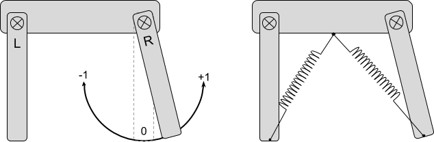
The object of our experiment will be a very simple two-legged creature. It has two legs, L and R, which are attached to the body by hinges. Thanks to two springs, they can be rotated. When the springs expand and contract, they retract and pull the legs, forcing them to turn. The creature does not know how to directly turn its legs, but can control the length of the springs, passing them a value in the range from -1 (compressed) to +1 (stretched).



Note: Moving complex bodies is a serious task. For the final project, I replaced Unity SpringJoint2D with DistanceJoint2D because they are more predictable. But I will still call them springs. For the more complex ragdoll shown in the animation, body parts will be rotated directly from the code.

Brain

Walking is not only a matter of finding the right angles for L and R. This is a long-term task that requires equally continuous leg movements. If we want to walk, then we need to provide a substantially compact and meaningful way to move our legs. The list of possible ways here is endless. For the sake of simplicity, the relaxation and compression of the springs will be controlled by two sinusoids.







The evolutionary process will adjust the L and R sinusoids so that the creature can walk. An example is shown in the animation above: the green and red sine waves control the legs L and R respectively.



Springs are creature-driven entities, they will be the target of our evolutionary computation. Each sinusoid has a period $$$p$ in the range of $$$m$ before $$$M$ and shifted along the x axis by $$$o$ . This means that the goal of evolution is to find two sets for these four parameters, which as a result give the best walking strategy.

Controller

In the existing system, we have several entities: legs, springs and sinusoids. To simplify the way of solving the problem, let's create the class LegController , which allows controlling the compression of the springs using values ​​from -1 to +1:







We rotate the legs by changing the length of the spring in FixedUpdate . This causes the connection to tighten or push the foot until it reaches the desired destination.

 public class LegController : MonoBehaviour { public DistanceJoint2D spring; private float contracted; private float relaxed; [Range(-1, +1)] public float position = +1; void Start () { float distance = spring.distance; relaxed = distance * 1.5f; contracted = distance / 2f; } void FixedUpdate () { spring.distance = linearInterpolation(-1, +1, contracted, relaxed, position); } public static float linearInterpolation(float x0, float x1, float y0, float y1, float x) { float d = x1 - x0; if (d == 0) return (y0 + y1) / 2; return y0 + (x - x0) * (y1 - y0) / d; } } 

Two foot controllers are constantly updated with the Creature class:

 public class Creature { public LegController left; public LegController right; public void Update () { left.position = // ... right.position = // ... } } 

In the next part of the tutorial, we will see how the Creature class evolves to include the creature's genome.

Fitness score

Evolution requires the assessment of the fitness of a being. This stage, although it seems rather trivial, is in fact incredibly complex. The reason is that the score we assign to each creature at the end of the simulation must correctly display exactly what we want to learn. If we fail to do this, then we will inevitably get poor results, and evolution will be stuck in local maxima.



My first attempt was to assess the fitness of the creature depending on the distance traveled from the starting point:

 private Vector3 initialPosition; public void Start () { initialPosition = transform.position; } public float GetScore () { return position.x - initialPosition.x; } 

This led to the least-effort walk strategy — dragging yourself across the floor:







I was not satisfied with this decision, because it did not seize one of the most important aspects of walking: maintaining balance. In the second attempt, I added a very serious bonus to all creatures who managed to stay on their feet:

 public float GetScore () { //   float walkingScore = position.x - initialPosition.x; //   bool headUp = head.transform.eulerAngles.z < 0+30 || head.transform.eulerAngles.z > 360-30; bool headDown = head.transform.eulerAngles.z > 180-45 && head.transform.eulerAngles.z < 180+45; return walkingScore * (headUp ? 2f : 1f) //  ,  UP * (headDown ? 0.5f : 1f) //     ,  DOWN ; } 

Since falling is incredibly simple, this function of fitness encouraged beings capable of maintaining good balance. However, she did not really encourage them to walk. The fall was estimated too strictly, and evolution did not feel bold enough to risk it.







To compensate for this, I tried to give impetus to the fact that maintaining balance was evaluated independently of walking.

 return walkingScore * (headDown ? 0.5f : 1f) + (headUp ? 2f : 0f) ; 

In all my attempts, creatures came to an awkward, but very functional solution:

Conclusion

In this part, we became acquainted with the body of the creature that will be used in the simulation. If you choose the design meaningfully, then evolution will work regardless of body type. It is worth noting that in my first attempt a much more complex body was used, in which four interconnected springs were used. It did not work very well because evolution was abusing the instability of the Box2D constraints, forcing the creature to fly at high speed. Yes, evolution likes to cheat, and very much.



In the third part of the tutorial, we will focus on the correct presentation and mutations of the creature's genome. The basis of this technique is the use of a form that is amenable to evolutionary computing.

Part 3. Genotype.

When we consider a task through the lens of evolution, we always need to take into account two sides of the coin: the phenotype and the genotype . In the previous section, we looked at the creation of the body of a being and its brain. Now it's time to focus on its genotype, that is, the method of presentation, transmission and mutation of such information.

Genome

As stated above, each leg is controlled by a sine wave. $$$s$ set by four parameters: $$$m$ , $$$M$ , $$$p$ and $$$o$ , i.e:

$$

$$s = \ frac {M-m} {2} \ left (1 + sin \ left (\ left (t + o \ right) \ frac {2 \ pi} {p} \ right) \ right) + m$$

This is just an ordinary sinusoid with a period $$$p$ in the range of $$$m$ before $$$M$ and offset along the x axis by $$$o$ .



The task of learning to walk has now become the task of finding a point in space with 8 dimensions (4 for each foot). Let's start creating the genome for one leg. It will be stored in a structure called GenomeLeg . It wraps four necessary parameters and provides an opportunity to evaluate the sinusoid it represents:

 [System.Serializable] public struct GenomeLeg { public float m; public float M; public float o; public float p; public float EvaluateAt (float time) { return (M - m) / 2 * (1 + Mathf.Sin((time+o) * Mathf.PI * 2 / p)) + m; } } 

Now we need to wrap the two GenomeLeg into a single structure that will store the entire genome:

 [System.Serializable] public struct Genome { public GenomeLeg left; public GenomeLeg right; } 

At this stage, we have a complete structure defining the creature’s walking strategy. This allows us to complete the Creature class, which we left in the previous section:

 public class Creature { public Genome genome; public LegController left; public LegController right; public void Update () { left.position = genome.left.EvaluateAt(Time.time); right.position = genome.right.EvaluateAt(Time.time); } } 

Cloning

The very basis of evolution is the concept of genome transmission and mutation. For evolution to work, we need to create copies of the genome and apply random mutations to them. Let's start by adding the Clone method to the GenomeLeg structure:

 public GenomeLeg Clone () { GenomeLeg leg = new GenomeLeg(); leg.m = m; leg.M = M; leg.o = o; leg.p = p; return leg; } 

And also to the Genome structure:

 public Genome Clone () { Genome genome = new Genome(); genome.left = left.Clone(); genome.right = right.Clone(); return genome; } 

It is worth noting that since they are small structures (shallow structs) , the Clone method is not required. Structures are treated as primitive types: they are always copied when they are transmitted or assigned.

Mutation

The most interesting part of this tutorial is obviously the mutations. Let's start with a simple one: mutate the Genome structure. We randomly select a leg and apply a mutation to it:

 public void Mutate () { if ( Random.Range(0f,1f) > 0.5f ) left.Mutate(); else right.Mutate(); } 

Now we need to take the leg's genome and apply a random mutation that could potentially improve its fitness. This can be done in an infinite number of ways. The one I chose for the tutorial simply selects a random parameter and changes it by a small amount:

 public void Mutate () { switch ( Random.Range(0,3+1) ) { case 0: m += Random.Range(-0.1f, 0.1f); m = Mathf.Clamp(m, -1f, +1f); break; case 1: M += Random.Range(-0.1f, 0.1f); M = Mathf.Clamp(M, -1f, +1f); break; case 2: p +=Random.Range(-0.25f, 0.25f); p = Mathf.Clamp(p, 0.1f, 2f); break; case 3: o += Random.Range(-0.25f, 0.25f); o = Mathf.Clamp(o, -2f, 2f); break; } } 

The Mutate method contains a lot of magic numbers - constants that appear from nowhere. Although it would be logical to limit the values ​​of our parameters, setting the mutation volumes, but here it is rather inefficient. A more sensible way would be to fine tune the parameters according to how close we are to the solution. When we are close to the goal, we need to slow down so as not to jump over the right solution and not to miss it. This aspect, often called adaptive learning rate , is an important stage of optimization that will not be considered in the tutorial.



It is also worth noting that changing values ​​by small values ​​can also prevent a better solution from being found. It is better to choose an approach in which one of the parameters is randomly replaced.

Conclusion

In this section, we explained how to present the behavior of a previously created creature in such a way that it can be controlled through evolutionary computing techniques.



In the next part, we will complete the evolution tutorial, showing the last necessary fragment: the evolution cycle itself.

Part 4. Cycle.

Our adventure of mastering the power of evolution comes to an end. In the previous three parts of the tutorial, we created a bipedal body and a mutated genome that determines its behavior. It remains for us to implement the evolutionary computation itself in order to find a successful walking strategy.

Evolution cycle

Evolution is an iterative process. We use korutina to ensure the continuation of such a cycle. In short, we will start with a certain genome and create several mutated copies. For each copy, we will create an instance of the creature and test its operation in the simulation. Then we take the genome of the most successful creature and repeat the iteration.

 public int generations = 100; public float simulationTime = 15f; public IEnumerator Simulation () { for (int i = 0; i < generations; i ++) { CreateCreatures(); StartSimulation(); yield return new WaitForSeconds(simulationTime); StopSimulation(); EvaluateScore(); DestroyCreatures(); yield return new WaitForSeconds(1); } } 

Simulation

To test the success of the creature’s walk, we need to create its body and give it enough time to move. To simplify the work, let's imagine that there is a fairly long floor in the game scene. We will create instances of creatures on top of it, at a considerable distance so that they do not affect each other. The code below performs exactly this task, placing creatures (stored in prefabs) at a certain distance .

 public int variations = 100; private Genome bestGenome; public Vector3 distance = new Vector3(50, 0, 0); public GameObject prefab; private List<Creature> creatures = new List<Creature>(); public void CreateCreatures () { for (int i = 0; i < variations; i ++) { //    Genome genome = bestGenome.Clone().Mutate(); //    Vector3 position = Vector3.zero + distance * i; Creature creature = Instantiate<Creature>(prefab, position, Quaternion.identity); creature.genome = genome; creatures.Add(creature); } } 

The CreateCreatures feature CreateCreatures track of all created creatures so that they can be manipulated more easily. To improve management, we will disable the Creature script in the creature prefab. Because of this, the creature will not move. Then we can start and stop the simulation using the following functions.

 public void StartSimulation () { foreach (Creature creature in creatures) creature.enabled = true; } public void StopSimulation () { foreach (Creature creature in creatures) creature.enabled = false; } public void DestroyCreatures () { foreach (Creature creature in creatures) Destroy(creature.gameObject); creatures.Clear(); } 

Fitness score

Evolution is about assessing fitness. After the simulation is completed, we cycle around all the creatures and get their final estimate. We are tracking the best creature so that you can mutate it in the next iteration.

 private float bestScore = 0; public void EvaluateScore () { foreach (Creature creature in creatures) { float score = creature.GetScore(); if (score > bestScore) { bestScore = score; bestGenome = creature.genome.Clone(); } } } 

Improvements

The attentive reader may have noticed that the technique described in this article depends on several parameters. Namely: generations , simulationTime and variations . They represent, respectively, the number of simulated generations, the duration of each simulation and the number of variations created in each generation. However, an even more attentive reader might also notice that the strategy used is poisoned by implied assumptions. They are the result of too simplified selected characteristics of the structure, which are now becoming hard constraints. Therefore, the results of a one-hour program and a month-running program will differ. In this section, I will try to solve problems with some of these limitations by creating more reasonable alternatives that you can implement yourself.

• Top K genomes. Genomes starting the next generation are the best of all generations. This means that if the current generation cannot improve fitness, then the next generation will start from the same genome. The obvious trap here is that we can get stuck in a cycle in which the same genome is simulated again and again, without any reasonable improvement. A possible solution would be to always take the best genome from the current run. The disadvantage of this approach is that fitness can decrease if none of the mutations bring any improvements. A more reasonable approach would be to select the best k genomes from each generation, and use them as the basis for the next iteration. You can add the unmutated best genome of the previous generation, so that the fitness does not deteriorate, but you can also find the best solutions.
• Adaptive learning speed. With each mutation of the genome, we change only one parameter of the leg and by a certain amount. Only mutations move us in the parameter space in which our solution lies. The speed with which we are moving is very important: if we move too far, we can jump over the decision, but if we move too slowly, then we can not get out of local maxima. The number of mutations performed ( learning rate ) of the genome must be related to the speed with which the score improves. The animation below shows how significant the effect of various strategies on the speed of convergence can be.

• Early completion. It is easy to see that some simulations lead us to a dead end. Every time a creature rolls onto its back, it will never be able to get back on its feet. A good algorithm should recognize them and interrupt such simulations to save resources.
• Changing the function of fitness. If what you want to learn is difficult enough, then perhaps it is worth doing it in stages. This can be realized by gradually changing the function of fitness. This way we can focus our training efforts on a simple task.
• A few checks. When it comes to physics simulation, there is a chance that you will never get one result twice. There is a good way to create several instances of a creature with the same genome under the same conditions, and then average their scores in order to get a more reliable estimate.

Conclusion

In this tutorial we got acquainted with evolutionary calculations and dealt with their work. This topic is incredibly broad, so take this article as a general introduction.



The full Unity package for this project can be downloaded here .