Applying recurrent layers to solve multiple paths

Story

Recurrent layers were invented back in the 80s by John Hopfield. They formed the basis of artificial associative neural networks (Hopfield networks) developed by him. Today, recurrent networks are widespread in the tasks of processing sequences: natural languages, speech, music, video sequence, and so on.

Task

As part of the task of hierarchy reinforcement learning, I decided to predict not one agent’s action, but several, using for this purpose a pre-trained network capable of predicting a sequence of actions. In this article, I will show how to implement the “sequence to sequence” algorithm for training this very network, and in the following, I will try to tell you how to use it in Q-learning training.

Environment

Imagine a small 2D game world, 5x5 cells. Each cell will occupy either an object or an empty space.

')



Before our network we set the task: to issue a sequence of actions from a given set of actions [“left”, “right”, “up”, “down”, “take”, “attack”].



At the entrance it is necessary to submit the state of our world, consisting of 25 separate cells, each of which can take one value from the set: [“space”, “enemy”, “life”, “source point”, “destination point”].







You can display such a world in the form of a vector of dimension 6 * 25, and then compress the embedded algorithm. Such a model will be very sensitive to changes in the number of cells and objects in this world.



To get rid of such limitations, we can form the input layer as a sequence, where each element of this sequence is one object of our world. Thus, we will feed the input sequences of different lengths (for different sizes of the simulated world) and in the process of pre-training we will be able to expand the number of objects in our world.

Sequence to sequence

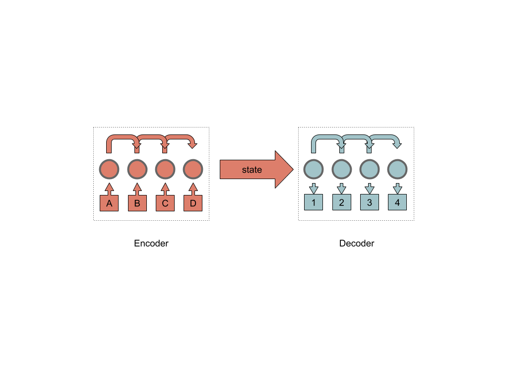
Sequence to sequence neural networks are two blocks encoder and decoder, and some kind of hidden layer of internal state connecting them.



In turn, the encoder consists of a chain of recurrent cells (in the implementation it can be one or several).



The most common today recurrent cell (in my subjective opinion) can be called the LSTM (Long short term memory) cell.







Without going into the implementation of LSTM, (I advise you to read more here ), I will briefly describe the principle of its work.



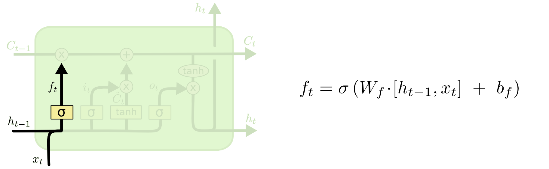
Three inputs C, H, X come to the LSTM input of the cell. The input of the “conveyor” C with possible linear modifications of the signal inside the cell. The first modification is the “gate”.







By processing the signal from the H and X inputs, the “gate” decides whether the signal coming through the pipeline C is passed. This happens by multiplying the signal C by the value of the sigmoid function with the parameters H, X, W, b.







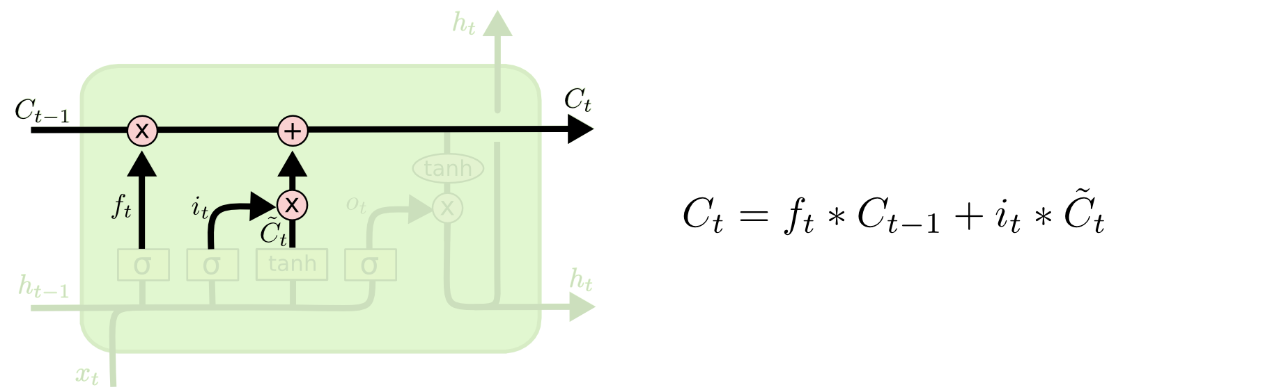
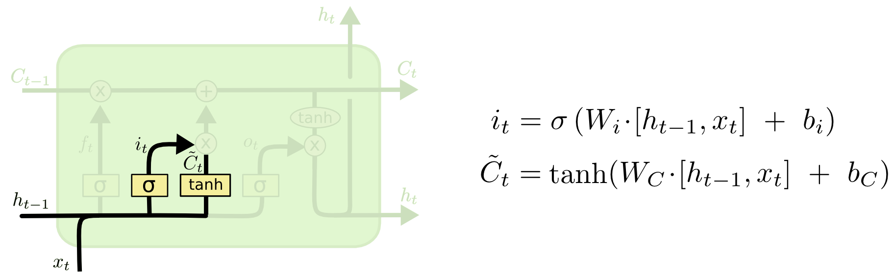
The next step is to decide which new information we are going to store in the cell state. This decision is made in two stages.







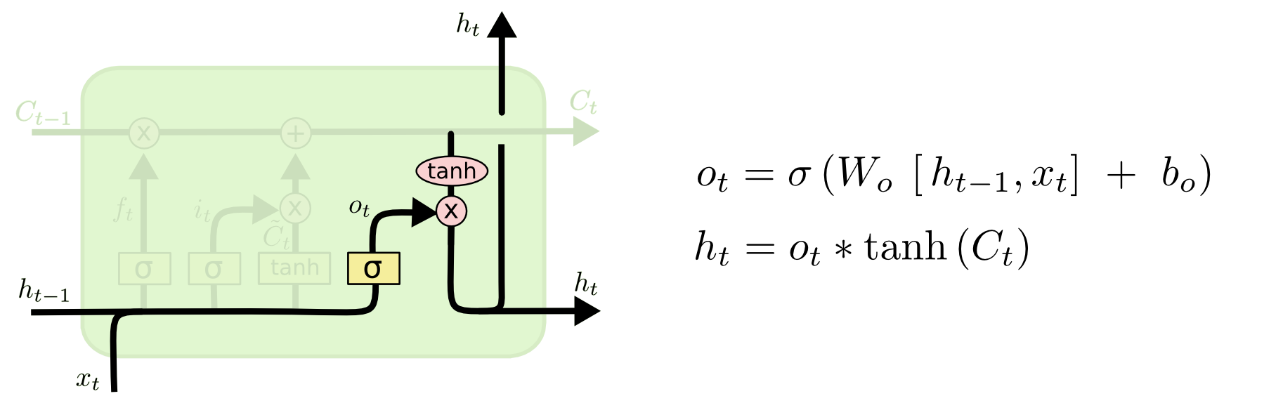
To begin with, the second sigmoid layer, called the “input gate layer”, decides which values ​​we will update. Then the tanh layer creates a vector of candidate values ​​of the output layer C, which can be added to the state. In the next step, the cell combines the signal going through the “pipeline” C, with the resulting one, to create an updated state. Finally, we need to decide what will be at the H output of our cell. This conclusion will be based on the state of our cell, but with this one a filter will pass. First, the cell will pass a signal through the sigmoid layer, which decides which parts of the state of the cell we are going to output. Then multiply it by the value of the “pipeline” C passing through the tanh function.



You can also read about LSTM on Habré .



Thus, collecting several LSTM cells in a “chain”, we can predict a certain state, based on previous predictions in the chain.



There are many techniques that help improve the convergence of such networks, for example, the technique of bidirectional cells. By arranging the cells in two rows so that one row monitors the state of the previous cell, and the other one follows the state of the cell after it, you can take into account not only the word that was before the predicted one, but also the next one. Also use “accents” or attention (attention) to determine the keywords in the proposal.

Implementation

I will “collect” the neural network with TensorFlow and the python language. Also for this article, I wrote a small class to simulate the world.



The first thing to do is to define the input layers:

self.input_data_input = tf.placeholder(tf.int32, [None, None], name='input') self.targets = tf.placeholder(tf.int32, [None, None], name='targets') self.learning_rate_input = tf.placeholder(tf.float32, name='learning_rate') self.target_sequences_length_input = tf.placeholder(tf.int32, (None,), name='target_sequences_length') self.max_target_sequences_length = tf.reduce_max(self.target_sequences_length_input, name='max_target_len') self.source_sequences_length_input = tf.placeholder(tf.int32, (None,), name='source_sequences_length') 

Next, create an encoder layer.



Here it should be said that the embedding mechanism is used to reduce the dimension, the mechanics of its implementation is already present in TensorFlow.

 # 1. Encoder embedding encoder_embed_input = tf.contrib.layers.embed_sequence(input_data_input, vocabulary_size, TF_FLAGS.FLAGS.encoding_embedding_size) # 2. Construct the encoder layer encoder_cell = tf.contrib.rnn.MultiRNNCell([self.make_cell() for _ in range(TF_FLAGS.FLAGS.num_layers)]) enc_output, enc_state = tf.nn.dynamic_rnn(encoder_cell, encoder_embed_input, sequence_length=source_sequences_length_input, dtype=tf.float32) 

We create rnn cell and add them to our network.

 dec_cell = tf.contrib.rnn.LSTMCell(TF_FLAGS.FLAGS.rnn_size, initializer=tf.random_uniform_initializer(-0.1, 0.1, seed=2)) 

More details you can see the video from TFSummit 2017 .



The output of our subnet will consist of the output (pipeline) of the last RNN cell and its hidden state. We only need a state.

Go to the decoder.



As in the decoder, you need to prepare an embedding layer.

 # 1. Decoder Embedding target_vocab_size = self.vocabulary_size decoder_embeddings = tf.Variable(tf.random_uniform([target_vocab_size, TF_FLAGS.FLAGS.decoding_embedding_size])) decoder_embed_input = tf.nn.embedding_lookup(decoder_embeddings, decoder_input) 

Next, create the first layer with recurrent cells and project their outputs onto a fully connected perceptron for further classification of the results.

 # 2. Construct the decoder layer dec_cell = tf.contrib.rnn.MultiRNNCell([self.make_cell() for _ in range(TF_FLAGS.FLAGS.num_layers)]) # 3. Dense layer to translate the decoder's output at each time # step into a choice from the target vocabulary output_layer = Dense(target_vocab_size, kernel_initializer=tf.truncated_normal_initializer(mean=0.0, stddev=0.1)) 

The cell outputs are fed to a fully connected layer of the classifier.



In the decoder, we will have two branches of the graff:



The first branch is for training, the other is for processing final tasks.

For training, we need to remove the last character from the target (those that we want to get at the output of the decoder) sequences and add "GO" at the beginning of each target sequence. This is necessary, since we will train each cell separately and for each of them it is necessary to send the correct input signal, and not the signal from the neighboring learning cell.



An assistant is needed to implement the TensorFlow decoder layer. In essence, this is an iterator that preprocesses the input data.



Create an assistant and a dynamic decoder for learning.

 # Helper for the training process. Used by BasicDecoder to read inputs. training_helper = tf.contrib.seq2seq.TrainingHelper(inputs=decoder_embed_input, sequence_length=target_sequences_length, time_major=False) # Basic decoder training_decoder = tf.contrib.seq2seq.BasicDecoder(dec_cell, training_helper, encoder_state, output_layer) # Perform dynamic decoding using the decoder training_decoder_output = tf.contrib.seq2seq.dynamic_decode(training_decoder, impute_finished=True, maximum_iterations=max_target_sequences_length)[0] 

We create an assistant and a dynamic decoder for processing final tasks.

 start_tokens = tf.tile(tf.constant([ua.UrbanArea.vacab_go_key], dtype=tf.int32), [TF_FLAGS.FLAGS.batch_size], name='start_tokens') # Helper for the inference process. inference_helper = tf.contrib.seq2seq.GreedyEmbeddingHelper(decoder_embeddings, start_tokens, ua.UrbanArea.vacab_eos_key) # Basic decoder inference_decoder = tf.contrib.seq2seq.BasicDecoder(dec_cell, inference_helper, encoder_state, output_layer) inference_decoder_output = tf.contrib.seq2seq.dynamic_decode(inference_decoder, impute_finished=True, maximum_iterations=max_target_sequences_length)[0] 

Next, add our loss function.



For sequences in TensorFlow there is a cross-entropy function, with which we will input the rnn output of the network and training examples to the input.

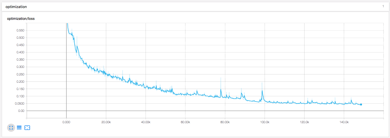
 training_logits = tf.identity(training_decoder_output.rnn_output, 'logits') _ = tf.identity(inference_decoder_output.sample_id, name='predictions') # Create the weights for sequence_loss masks = tf.sequence_mask(self.target_sequences_length_input, self.max_target_sequences_length, dtype=tf.float32, name='masks') with tf.name_scope("optimization"): # Loss function self.cost = tf.contrib.seq2seq.sequence_loss(training_logits, self.targets, masks) tf.summary.scalar("loss", self.cost) 

Gradient descent and Adam optimizer will update the scale values.

 # Optimizer optimizer = tf.train.AdamOptimizer(self.learning_rate_input) # Gradient Clipping gradients = optimizer.compute_gradients(self.cost) capped_gradients = [(tf.clip_by_value(grad, -5., 5.), var) for grad, var in gradients if grad is not None] self.train_op = optimizer.apply_gradients(capped_gradients) 

That's all, it is enough to get several hundred training data from our simulator and start the training session.



Epoch 1/100 Batch 20/65 Loss: 1.170 Validation loss: 1.082 Time: 0.0039s

Epoch 1/100 Batch 40/65 Loss: 0.868 Validation loss: 0.950 Time: 0.0029s

Epoch 1/100 Batch 60/65 Loss: 0.939 Validation loss: 0.794 Time: 0.0031s

...

Epoch 99/100 Batch 60/65 Loss: 0.136 Validation loss: 0.403 Time: 0.0030s

Epoch 100/100 Batch 20/65 Loss: 0.149 Validation loss: 0.430 Time: 0.0037s

Epoch 100/100 Batch 40/65 Loss: 0.110 Validation loss: 0.423 Time: 0.0031s

Epoch 100/100 Batch 60/65 Loss: 0.153 Validation loss: 0.397 Time: 0.0031s





As a result, you can get a sequence of steps to walk through our virtual labyrinth.



The yellow sequence highlighted by the algorithm, green - the sequence proposed by an artificial neural network.







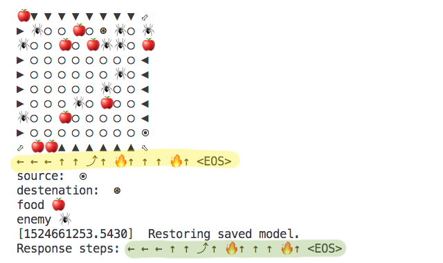
I also added some visualization to the training.







You can see the complete solution in my github repository.