Autopilot on your own. Part 1 - we collect the training data

Hi, Habr. This is a post-report-tutorial about unmanned vehicles - how to (start) make your own without spending on equipment. All code is available on github , and among other things, you will learn how to easily generate such cool images:

Go!

In short

Summary for those familiar with the topic: Traditionally, a specially equipped car with a sufficiently informative CAN bus and interface to it was expensive to recruit a training set for the autopilot based on machine learning. We will do it easier and for free - we will type the same data in essence just from the smartphone on the windshield. Fits any car, no equipment modifications. In this series, we calculate the turn of the steering wheel at each moment in time by video. If everything is clear in this paragraph, you can jump over the introduction to the essence of the approach .

What-why-why in more detail

So, a couple of years ago, without serious resources of a large corporation on the topic of autopilots, it was impossible to turn around - the LIDAR sensor alone was worth tens of thousands of dollars , but the recent revolution in neural networks changed everything. Startups of several people with the simplest sensor sets from a pair of webcams compete on equal terms in terms of the quality of the result with famous brands. Why not try us too, especially since so many high-quality components are already in the public domain .

The autopilot converts sensor data into control actions — the steering turn and the required acceleration / deceleration. In a laser rangefinder system like Google’s, it might look like this:

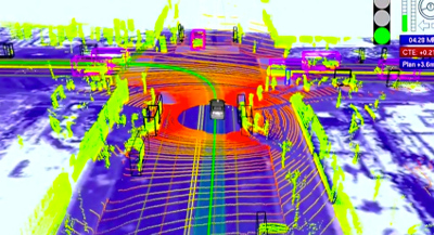
The simplest version of the sensor is a video camera “looking” through the windshield. We will work with him, because everyone already has a camera on the phone.

For calculating control signals from raw video, convolutional neural networks work well, but, like any other machine learning approach, they need to be taught to predict the correct result. For training, you need (a) to choose a model architecture and (b) to form a training set that will demonstrate models of different input situations and "correct answers" (for example, the steering angle and the position of the gas pedal) for each of them. Data for a training sample is usually recorded from races where the machine is operated by a person. That is, the driver demonstrates the robot how to operate the machine.

There are enough good neural networks architectures in the public domain , but the situation is more sad with data: firstly, there is simply not enough data, secondly, almost all samples come from the USA , and on our roads there are a lot of differences from those places .

The lack of open data is easily explained. First of all, data is no less valuable asset than expertise in algorithms and models, so no one is in a hurry to share:

The rocket engine is the data.

Andrew Ng

Secondly, the process of collecting data is not cheap, especially if you act head-on. A good example is Udacity . They specially selected a car model where the steering and gas / brake are tied to a digital bus, made an interface to the bus, and read data from there directly. Plus approach - high quality data. Minus - a serious cost, cutting off the vast majority of non-professionals. After all, not every modern car even writes all the information we need to CAN , and we’ll have to tinker with the interface.

We will proceed easier. We record the "raw" data (for now it will be just a video) with a smartphone on the windshield as a DVR, then use the software to "squeeze" the necessary information from there - the speed of movement and turns, on which the autopilot can already be trained. As a result, we get an almost free solution - if there is a phone holder on the windshield, just press a button to type training data on the way to work.

In this series - "squeezer" angle of rotation from the video. All steps are easy to repeat on your own using the code on github .

Task

We solve the problem:

• There is a video from the camera, rigidly fixed to the car (ie, the camera does not hang out).
• It is required for each frame to find out the current steering angle.

Expected Result:

Immediately just simplify - instead of the steering angle, we calculate the angular velocity in the horizontal plane. This is roughly equivalent information if we know the translational speed, which we will deal with in the next series.

Decision

The solution can be assembled from publicly available components by slightly modifying them:

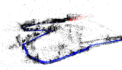
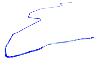
We restore the trajectory of the camera

The first step is to restore the camera's trajectory in three-dimensional space using the SLAM library for video (simultaneous localization and mapping, simultaneous localization and mapping). At the output for each (almost, see the nuances) of the frame, we get 6 position parameters: 3D offset and 3 orientation angles .

In the code, the optical_trajectories module is responsible for this part optical_trajectories

Nuances:

• When recording video, do not chase the maximum resolution - beyond a certain threshold, it only hurts. My settings around 720x480 work well.
• The camera will need to be calibrated ( instructions , theory — parts 1 and 2 are relevant ) at the same settings with which the video from the race was recorded .
• The SLAM system needs a "good" sequence of frames, for which you can "hook" as a starting point, so part of the video at the beginning, until the system is "hooked" will not be annotated. If localization on your video does not work at all, either calibration problems are likely (try to calibrate several times and look at the variation of the results), or video quality problems (too high resolution, too much compression, etc.).
• There may be breakdowns in the tracking system by the SLAM system, if too many key points are lost between adjacent frames (for example, glass was momentarily flooded with a splash from a puddle). In this case, the system will be reset to its original non-localized state and will be localized again. Therefore, from one video you can get several trajectories (not intersecting in time). The coordinate systems in these trajectories will be completely different.
• The specific library ORB_SLAM2, which I used, gives not very reliable results on translational displacements, so we ignore them for now, but determine the rotation quite well, we leave them.

Determine the plane of the road

The trajectory of the camera in three-dimensional space is good, but it does not directly answer the final question whether to turn left or right, and how quickly. After all, the SLAM system does not have the concepts of "road plane", "up-down", etc. This information must also be obtained from the "raw" 3D trajectory.

A simple observation will help here: highways are usually stretched far further horizontally than vertically. There are of course exceptions , they will have to be neglected. And if so, you can take the nearest plane (ie, the plane, the projection on which gives the minimal reconstruction error) of our trajectory beyond the horizontal plane of the road.

We select the horizontal plane by an excellent method of principal components along all 3D points of the trajectory — we remove the direction with the smallest eigenvalue, and the remaining two will give the optimal plane.

The optical_trajectories module is also responsible for the plane selection logic optical_trajectories

Nuance:

• From the essence of the main components, it is clear that apart from mountain roads, the selection of the main plane will work poorly if the car has been traveling in a straight line all the time, because then only one direction of a real horizontal plane will have a large range of values, and the range along the remaining perpendicular horizontal direction and vertically will be comparable.

  
  
  

  In order not to pollute the data with large errors from such trajectories, we check that the spread on the last main component is significantly (100 times) smaller than on the last but one. Non-past trajectories are simply thrown away.

  
  
  

Calculate the angle of rotation

Knowing the basis vectors of the horizontal plane v ₁ and v ₂ (the two main components with the largest eigenvalues ​​from the previous part), we project the optical axis of the camera onto the horizontal plane:

Thus, from the three-dimensional orientation of the camera, we obtain the vehicle heading angle (up to an unknown constant, since the axis of the camera and the axis of the car generally do not match). Since we are only interested in the intensity of rotation (i.e. angular velocity), this constant is not needed.

The angle of rotation between adjacent frames is given by school trigonometry (the first factor is the absolute value of the turn, the second is the sign that determines the direction to the left / right). Here, a _t means the projection vector a _horizontal at time t:

This part of the computation is also done by the optical_trajectories module. At the output we get a JSON file of the following format:

 { "plane": [ [ 0.35, 0.20, 0.91], [ 0.94, -0.11, -0.33] ], "trajectory": [ ..., { "frame_id": 6710, "planar_direction": [ 0.91, -0.33 ], "pose": { "rotation": { "w": 0.99, "x": -0.001, "y": 0.001, "z": 0.002 }, "translation": [ -0.005, 0.009, 0.046 ] }, "time_usec": 223623466, "turn_angle": 0.0017 }, ..... } 

Component values:

• plane - the basis vectors of the horizontal plane.
• trajectory - a list of items, one for each frame successfully tracked by the SLAM system.
  
  
  • frame_id - frame number in the source video (starting from 0).
  • planar_direction - projection of the off-axis on the horizontal plane
  • pose - camera position in 3D space
    
    
    • rotation - orientation of the optical axis in the unit quaternion format.
    • translation - offset.
  • time_use - time from the beginning of the video in microseconds
  • turn_angle - horizontal rotation relative to the previous frame in radians.

Remove noise

We are almost there, but the problem remains. Let's look at the resulting (for now) graph of angular velocity:

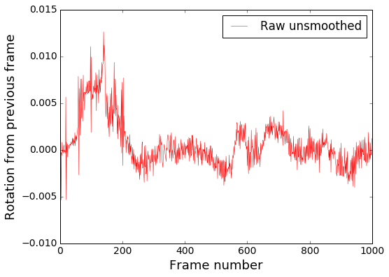
We visualize on video:

It is seen that in general, the direction of rotation is determined correctly, but a lot of high-frequency noise. We remove it with Gaussian blur , which is a low-pass filter.

Smoothing in the code is done by the smooth_heading_directions module

Result after the filter:

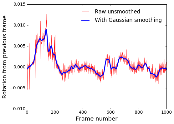
It is already possible to feed the learning model and rely on adequate results.

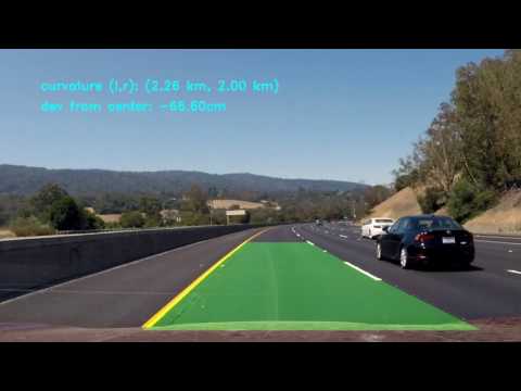
Visualization

For clarity, according to the data from the JSON files of the trajectories, you can impose a virtual steering wheel on the original video, as in the demos above, and check whether it is spinning correctly. This is the render_turning module.

It is also easy to build a frame schedule. For example, in an IPython laptop with matplotlib installed:

 import matplotlib %matplotlib inline import matplotlib.pyplot as plt import json json_raw = json.load(open('path/to/trajectory.json')) rotations = [x['turn_angle'] for x in json_raw['trajectory']] plt.plot(rotations, label='Rotations') plt.show() 

That's all for now. In the next series, we define the translational speed in order to train also speed control, but for now pull-requests are welcome.