An example of a vector implementation of a neural network using Python
The article discusses the construction of neural networks (with regularization) with calculations mainly vector-based method of Python. The article is close to the materials of the course Machine learning by Andrew Ng for quicker perception, but if you did not complete the course, nothing terrible, nothing specific is foreseen. If you have always wanted to build your neural network with preference and young lady vectors and regularization, but something is holding you back, now is the time.
This article is aimed at the practical implementation of neural networks, and it is assumed that the reader is familiar with the theory (so it will be omitted).
The code is commented in English, but it is unlikely that someone will have difficulties, since the main comments are also given in the article in Russian.
We will write code to search for optimal weights using scipy.optimize.fmin_cg, as well as independently, so the scripts will be universal.
')
We will immediately move on to practice, there are many articles on neural networks on Habré,
Software and dependencies
Python 3.4 (on 2.7 will also work with minor edits)
Numpy
SciPy (optional)
For convenience, all functions of the neural network will be rendered into separate module network.py
The first thing you want to do is create a fully connected neural network. In fact, this means that we need to initialize the Theta θ weights matrices with random values from -1 to 1.
Since we are creating functions inside the network class, the function will actually have one layers variable, which contains the number of layers and neurons in the created network in the list format. For example [10, 5, 5, 1] means a network with ten input neurons, two hidden layers of 5 neurons each and an output layer with one neuron.
Since the size of the variable layers is unlikely to exceed a few dozen elements even in the most complex neural network, in this case, apply a for loop.
As a result, we want to get a list theta whose elements will be matrices with weights.
At this stage we need to calculate the output signal of the neural network using the weights initialized in the previous step.
In short, using the np.vectorize command, the function can now take and read matrices of values. For example, for each element of the 10x1 matrix, a logistic function will be calculated, and a matrix of values with a dimension of 10x1 will be returned.
From the important I want to note that we add a column of bias after we applied the activation function to the sum of the products. This means that the bias is always equal to one, and not the logistic function of one (which is 0.73)
In addition, in the final matrix of activation functions the bias is present in all layers except the output layer, it contains only the output signals of the neural network (respectively, the dimension of the matrix = number of examples * number of neurons in the output layer).
For those who are not familiar with python, I note that the runAll function does not transfer copies of variables (for example, the neural network itself nn ) but references to them, so when we change the variable nn ['z'] = z we change our network nn despite by not passing the nn variable back.
As a result, this function ( runAll ) will return to us the matrix of the output signals of the network (its dimensionality is the number of output neurons * 1) and will change the matrices z and a in the variable neural network.
The error of the output signal of the neural network with regularization is calculated by the following formula
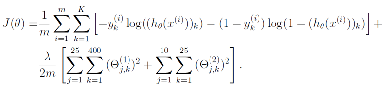
Picture taken from Machine Learning course materials.
m is the number of examples, K is the number of output neurons of the neural network, h0 (xi) is the vector of output values of the neural network, θ is the weights matrix, where θ ^ 1 is the weights matrix for the first hidden layer, lambda is the regularization coefficient.
If it seems to you rather scary and incomprehensible, it is normal :), in essence, it is decomposed into 2 components, with which we will work.
A detailed and understandable explanation of the essence of this formula will stretch out, and I am not sure that it is necessary for such a prepared public, so for now let us omit it, but write, if necessary, add.
Actually the error function will return us a single value in the float format, which will characterize how correctly our neural network calculates the output signal.
The function returns a neural network error for a given matrix X of input parameters.
Calculate the first part of the formula, the network error itself.
We consider regularization
We assume a cycle through the array with theta matrices, since it is assumed that we have a very limited number of layers, and the performance will not suffer much damage.
We remove from the regularization the connection with the bias, since it may well be of great importance if we need to shift the logistics function along the X axis.
At this stage, we can create a neural network, calculate the output signal and error, now it is only necessary to calculate the gradient and implement the weights correction algorithm.
At this step, we can not do without a cycle of incoming vectors and in order to speed up the calculation of the gradient a little, we carry out a maximum of operations before the cycle. For example, in the previous steps, we specifically designed the runAll function so that it calculates a matrix of input values, and not vectors (strings) individually, at this stage we will calculate the output values in advance, then we will access them in a loop. According to experimental measurements, these features speed up the function by an additional 25%
We use the reverse cycle through the layers of the neural network from the last to the first, since we need to calculate the error and transfer it back to the layer to calculate the next one, etc.
The main difficulty is not to get confused in the indices of variables. For example, in most documentation on neural networks for example a three-layer network (with one hidden layer), the delta of the output layer will have index 3, it is clear that in this case the sheet should consist of four elements, while the gradient sheet consists of 3 elements.
The function returns a sheet whose elements are matrices whose dimensions coincide with the dimension of theta matrices.
Moreover, this function is lambda, it is nothing but a derivative of the activation function (sigmoid), so if you want to replace the activation function, also change the derivative
Now we can test our neural network and even try to teach it something :)
To begin with we will teach our network simple segmentation, all values within [0; 5) is zero, [5; 9] is one
Result. Neural network output before training, training and after training. It is seen that after training, the first five values are closer to zero, the second five are closer to one.
In the previous example, the training was controlled by the function fmin_cg, but now we will change theta (network weight) independently.
Let's set a simple task, to distinguish an upward trend from a downward one. Neural network input will be fed 4 numbers, if they are consistently increased, this is one, if they decrease, this is zero.
After 400 iterations (about 1 min.) For some reason, the last test case has the highest error (output of the neural network 0.13), most likely in this case it would help to add training data to improve the quality.
In the cycle we change theta in order to achieve the maximum result. It turns out that we are gliding to the local minimum of the function (and if we added a gradient, then we would go to the local maximum). The variable alf, often called the “learning rate”, is responsible for how much we will change theta in each iteration. Moreover, if you set the alpha parameter too large, the network error may even increase or jump up and down as the function will simply step over the local minimum.
As you can see, the entire neural network consists of a single variable of the type dict, so it is easy to make it a secondary one, and save it in a simple text file and also restore it for future use.
Perhaps the next post will be on how to speed up this code (and any other written in Python) using GPU computing.
UPD
Thanks to everyone who is a plus.
This article is aimed at the practical implementation of neural networks, and it is assumed that the reader is familiar with the theory (so it will be omitted).
The code is commented in English, but it is unlikely that someone will have difficulties, since the main comments are also given in the article in Russian.
We will write code to search for optimal weights using scipy.optimize.fmin_cg, as well as independently, so the scripts will be universal.
')
What vectors are we talking about and why are they needed?
Suppose a simple task is to add in pairs the elements of two one-dimensional arrays. We can solve this problem in a loop with enumeration of all array values or add two vectors. Consider the following code.
On a simple laptop, the cycle is processed in an average of 4 seconds. 40 mil seconds Vectors add up in 0.02 sec.
Approximately the same difference in speed and with other arithmetic operations. Not to mention the visibility of the code.
import numpy as np import time A = np.random.rand(1000000, 1) # 1 . 1 float B = np.random.rand(1000000, 1) # ---- C1 = np.empty((1000000, 1)) # 1 . 1 C2 = np.empty((1000000, 1)) # 1 . 1 start = time.time() for i in range(0, len(A)): C1[i] = A[i] * B[i] # A, B C print(time.time() - start) start = time.time() C2 = A + B # print(time.time() - start) if (C1 == C2).all(): # print('Equal!') On a simple laptop, the cycle is processed in an average of 4 seconds. 40 mil seconds Vectors add up in 0.02 sec.
Approximately the same difference in speed and with other arithmetic operations. Not to mention the visibility of the code.
We will immediately move on to practice, there are many articles on neural networks on Habré,
for example these
Software and dependencies
Python 3.4 (on 2.7 will also work with minor edits)
Numpy
SciPy (optional)
For convenience, all functions of the neural network will be rendered into separate module network.py
Networking
The first thing you want to do is create a fully connected neural network. In fact, this means that we need to initialize the Theta θ weights matrices with random values from -1 to 1.
Since we are creating functions inside the network class, the function will actually have one layers variable, which contains the number of layers and neurons in the created network in the list format. For example [10, 5, 5, 1] means a network with ten input neurons, two hidden layers of 5 neurons each and an output layer with one neuron.
def create(self, layers): theta=[0] for i in range(1, len(layers)): # for each layer from the first (skip zero layer!) theta.append(np.mat(np.random.uniform(-1, 1, (layers[i], layers[i-1]+1)))) # create nxM+1 matrix (+bias!) with random floats in range [-1; 1] nn={'theta':theta,'structure':layers} return nn Since the size of the variable layers is unlikely to exceed a few dozen elements even in the most complex neural network, in this case, apply a for loop.
As a result, we want to get a list theta whose elements will be matrices with weights.
Why do we initialize theta [0] = 0?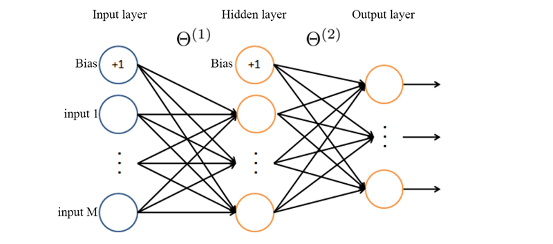
Picture from materials of the course Machine Learning, with modifications
In the field of neural networks, it is accepted to call the θ1 matrix of weights from input data (input) to the first neural layer. Since we do not have any layers up to the Input layer, there is no zero weight matrix either.
Picture from materials of the course Machine Learning, with modifications
In the field of neural networks, it is accepted to call the θ1 matrix of weights from input data (input) to the first neural layer. Since we do not have any layers up to the Input layer, there is no zero weight matrix either.
What is theta [1], theta [2], ..., theta [n]?
All matrices are compiled by one algorithm, so consider theta [1] for example. Theta [1] is a matrix in which the number of rows is equal to the number of neurons in the first hidden layer, and the number of columns is equal to the column for the bias (offset) + the number of neurons in the input layer.
That is, if we take the first row of the theta [1] matrix, then the zero element (read the zero column) will correspond to the weight of the bias, the other elements (columns) will correspond to the weights for communication with each element of the incoming layer.
That is, if we take the first row of the theta [1] matrix, then the zero element (read the zero column) will correspond to the weight of the bias, the other elements (columns) will correspond to the weights for communication with each element of the incoming layer.
What is Bias and why is it needed?
Bias is translated from English as “offset” and in fact this is what it means (always yours, Cap). Better than here I can hardly say, so I’ll just complete the translation.
Bias is almost always useful because it allows you to shift the activation function to the left or right , which can be extremely important for successful learning.
A simple example will help to understand. Imagine the simplest neural network without a hidden layer, only one incoming and 1 outgoing neuron
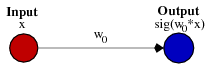
The output signal of the neural network is calculated by multiplying the weight of W0 by the signal X and applying the activation function (most often sigmoid) to the product.
An example of the functions that we obtain for different values of the weight W0
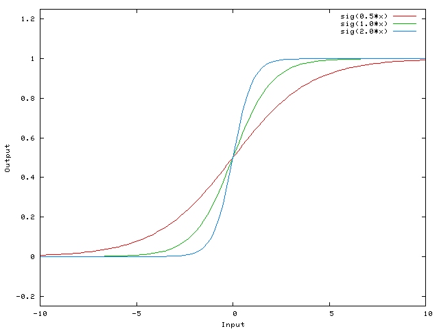
Changing the value of the weight W0 we change the slope of the curve, the degree of its steepness, this is convenient, but what if we want the outgoing signal to be 0 when X is 2? Just changing the slope of the curve will not work - it will not work to shift the entire curve to the right .
This is what Bias does. If we add Bias to our neural network, like this:
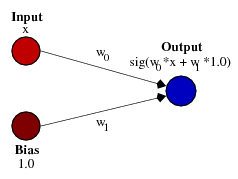
... then the output of our neural network will be considered sig (w0 * x + w1 * 1.0). Accordingly, our function will look like this when changing the weight of W1:
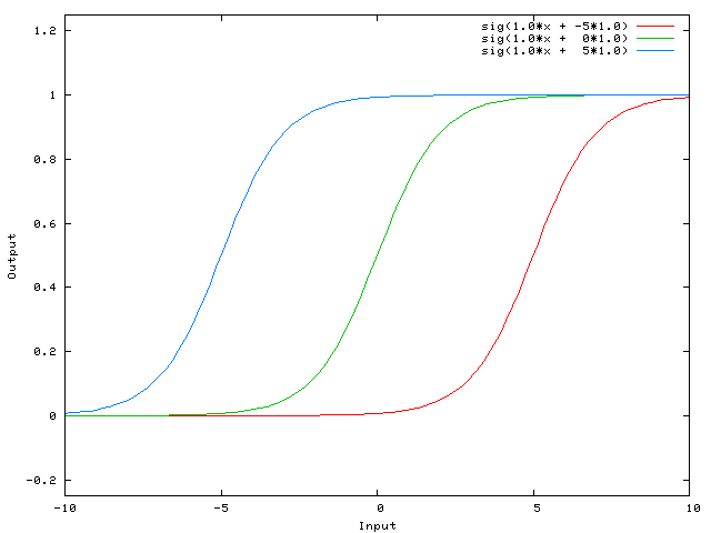
The weight of W1 equal to -5 will shift the curve to the right, therefore the output signal of the neural network will be equal to 0 with X equal to 2
Bias is almost always useful because it allows you to shift the activation function to the left or right , which can be extremely important for successful learning.
A simple example will help to understand. Imagine the simplest neural network without a hidden layer, only one incoming and 1 outgoing neuron
The output signal of the neural network is calculated by multiplying the weight of W0 by the signal X and applying the activation function (most often sigmoid) to the product.
An example of the functions that we obtain for different values of the weight W0
Changing the value of the weight W0 we change the slope of the curve, the degree of its steepness, this is convenient, but what if we want the outgoing signal to be 0 when X is 2? Just changing the slope of the curve will not work - it will not work to shift the entire curve to the right .
This is what Bias does. If we add Bias to our neural network, like this:
... then the output of our neural network will be considered sig (w0 * x + w1 * 1.0). Accordingly, our function will look like this when changing the weight of W1:
The weight of W1 equal to -5 will shift the curve to the right, therefore the output signal of the neural network will be equal to 0 with X equal to 2
Neural network outgoing signal calculation
At this stage we need to calculate the output signal of the neural network using the weights initialized in the previous step.
def runAll(self, nn, X): z=[0] m = len(X) a = [ copy.deepcopy(X) ] # a[0] is equal to the first input values logFunc = self.logisticFunctionVectorize() for i in range(1, len(nn['structure'])): # for each layer except the input a[i-1] = np.c_[ np.ones(m), a[i-1]]; # add bias column to the previous matrix of activation functions z.append(a[i-1]*nn['theta'][i].T) # for all neurons in current layer multiply corresponds neurons # in previous layers by the appropriate weights and sum the productions a.append(logFunc(z[i])) # apply activation function for each value nn['z'] = z nn['a'] = a return a[len(nn['structure'])-1] More detailed description of variables
Matrix X format: rows - vectors of input values (input values), columns - elements of vectors.
Z - sheet with matrices of the sum of products of the activation function values from the previous layer and the weights connecting them with the current layer by the neuron. Incoming values do not need to use the activation function, they have no weights, so we skip z [0] and start with z [1]
a - sheet with matrices of activation function values
a [0] is a matrix containing a bias (a unit vector of dimension m * 1) and incoming vectors X, that is, its dimension is the number of rows in X * (1 + the number of columns in X). Accordingly, a [1] contains the matrix value of activation functions in the first hidden layer, its dimensionality is the number of rows in X * (1 + the number of neurons in the first hidden layer)
def logisticFunction(self, x): a = 1/(1+np.exp(-x)) if a == 1: a = 0.99999 #make smallest step to the direction of zero elif a == 0: a = 0.00001 # It is possible to use np.nextafter(0, 1) and #make smallest step to the direction of one, but sometimes this step is too small and other algorithms fail :) return a def logisticFunctionVectorize(self): return np.vectorize(self.logisticFunction) In short, using the np.vectorize command, the function can now take and read matrices of values. For example, for each element of the 10x1 matrix, a logistic function will be calculated, and a matrix of values with a dimension of 10x1 will be returned.
What are these conditions in the logisticFunction function?
In the code above, one important pitfall is associated with rounding (here you have to run into the front). Suppose that you are preparing a large network, many layers, many neurons, you initialize weights randomly and it turns out that the sum of products on the output layer for each neuron is very small, for example -40. The logistic function from -40 will happily return you a unit.
Next, we will need to calculate the error of our neural network and we will transfer this unit to calculate the logarithm from 1 - the output value [log (1-output)] is naturally the logarithm of the unit is not defined, but the error does not pop up, just our neural network will not train.
Next, we will need to calculate the error of our neural network and we will transfer this unit to calculate the logarithm from 1 - the output value [log (1-output)] is naturally the logarithm of the unit is not defined, but the error does not pop up, just our neural network will not train.
From the important I want to note that we add a column of bias after we applied the activation function to the sum of the products. This means that the bias is always equal to one, and not the logistic function of one (which is 0.73)
a[i-1] = np.c_[ np.ones(m), a[i-1]]; In addition, in the final matrix of activation functions the bias is present in all layers except the output layer, it contains only the output signals of the neural network (respectively, the dimension of the matrix = number of examples * number of neurons in the output layer).
For those who are not familiar with python, I note that the runAll function does not transfer copies of variables (for example, the neural network itself nn ) but references to them, so when we change the variable nn ['z'] = z we change our network nn despite by not passing the nn variable back.
As a result, this function ( runAll ) will return to us the matrix of the output signals of the network (its dimensionality is the number of output neurons * 1) and will change the matrices z and a in the variable neural network.
Neural network error
The error of the output signal of the neural network with regularization is calculated by the following formula
Picture taken from Machine Learning course materials.
m is the number of examples, K is the number of output neurons of the neural network, h0 (xi) is the vector of output values of the neural network, θ is the weights matrix, where θ ^ 1 is the weights matrix for the first hidden layer, lambda is the regularization coefficient.
If it seems to you rather scary and incomprehensible, it is normal :), in essence, it is decomposed into 2 components, with which we will work.
A detailed and understandable explanation of the essence of this formula will stretch out, and I am not sure that it is necessary for such a prepared public, so for now let us omit it, but write, if necessary, add.
What is the essence of regularization?
The second line of the formula is responsible for regularization, the larger the regularization parameter, the greater the neural network error (since the sum of two positive numbers occurs in the whole formula), therefore in the process of learning, to reduce the error, it will be necessary to reduce the neural network weights, that is, a high regularization coefficient will keep the weights of the neural network small.
Actually the error function will return us a single value in the float format, which will characterize how correctly our neural network calculates the output signal.
def costTotal(self, theta, nn, X, y, lamb): m = len(X) #following string is for fmin_cg computaton if type(theta) == np.ndarray: nn['theta'] = self.roll(theta, nn['structure']) y = np.matrix(copy.deepcopy(y)) hAll = self.runAll(nn, X) #feed forward to obtain output of neural network cost = self.cost(hAll, y) return cost/m+(lamb/(2*m))*self.regul(nn['theta']) #apply regularization The function returns a neural network error for a given matrix X of input parameters.
Calculate the first part of the formula, the network error itself.
def cost(self, h, y): logH=np.log(h) log1H=np.log(1-h) cost=-1*yT*logH-(1-yT)*log1H #transpose y for matrix multiplication return cost.sum(axis=0).sum(axis=1) # sum matrix of costs for each output neuron and input vector We consider regularization
def regul(self, theta): reg=0 thetaLocal=copy.deepcopy(theta) for i in range(1,len(thetaLocal)): thetaLocal[i]=np.delete(thetaLocal[i],0,1) # delete bias connection thetaLocal[i]=np.power(thetaLocal[i], 2) # square the values because they can be negative reg+=thetaLocal[i].sum(axis=0).sum(axis=1) # sum at first rows, than columns return reg We assume a cycle through the array with theta matrices, since it is assumed that we have a very limited number of layers, and the performance will not suffer much damage.
We remove from the regularization the connection with the bias, since it may well be of great importance if we need to shift the logistics function along the X axis.
Gradient calculation
At this stage, we can create a neural network, calculate the output signal and error, now it is only necessary to calculate the gradient and implement the weights correction algorithm.
At this step, we can not do without a cycle of incoming vectors and in order to speed up the calculation of the gradient a little, we carry out a maximum of operations before the cycle. For example, in the previous steps, we specifically designed the runAll function so that it calculates a matrix of input values, and not vectors (strings) individually, at this stage we will calculate the output values in advance, then we will access them in a loop. According to experimental measurements, these features speed up the function by an additional 25%
We use the reverse cycle through the layers of the neural network from the last to the first, since we need to calculate the error and transfer it back to the layer to calculate the next one, etc.
The main difficulty is not to get confused in the indices of variables. For example, in most documentation on neural networks for example a three-layer network (with one hidden layer), the delta of the output layer will have index 3, it is clear that in this case the sheet should consist of four elements, while the gradient sheet consists of 3 elements.
def backpropagation(self, theta, nn, X, y, lamb): layersNumb=len(nn['structure']) thetaDelta = [0]*(layersNumb) m=len(X) #calculate matrix of outpit values for all input vectors X hLoc = copy.deepcopy(self.runAll(nn, X)) yLoc=np.matrix(y) thetaLoc = copy.deepcopy(nn['theta']) derFunct=np.vectorize(lambda x: (1/(1+np.exp(-x)))*(1-(1/(1+np.exp(-x)))) ) zLoc = copy.deepcopy(nn['z']) aLoc = copy.deepcopy(nn['a']) for n in range(0, len(X)): delta = [0]*(layersNumb+1) #fill list with zeros delta[len(delta)-1]=(hLoc[n].T-yLoc[n].T) #calculate delta of error of output layer for i in range(layersNumb-1, 0, -1): if i>1: # we can not calculate delta[0] because we don't have theta[0] (and even we don't need it) z = zLoc[i-1][n] z = np.c_[ [[1]], z ] #add one for correct matrix multiplication delta[i]=np.multiply(thetaLoc[i].T*delta[i+1],derFunct(z).T) delta[i]=delta[i][1:] thetaDelta[i] = thetaDelta[i] + delta[i+1]*aLoc[i-1][n] for i in range(1, len(thetaDelta)): thetaDelta[i]=thetaDelta[i]/m thetaDelta[i][:,1:]=thetaDelta[i][:,1:]+thetaLoc[i][:,1:]*(lamb/m) #regularization if type(theta) == np.ndarray: return np.asarray(self.unroll(thetaDelta)).reshape(-1) # to work also with fmin_cg return thetaDelta The function returns a sheet whose elements are matrices whose dimensions coincide with the dimension of theta matrices.
Moreover, this function is lambda, it is nothing but a derivative of the activation function (sigmoid), so if you want to replace the activation function, also change the derivative
lambda x: (1/(1+np.exp(-x)))*(1-(1/(1+np.exp(-x)))) Testing
Now we can test our neural network and even try to teach it something :)
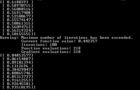
To begin with we will teach our network simple segmentation, all values within [0; 5) is zero, [5; 9] is one
nn=nt.create([1, 1000, 1]) lamb=0.3 cost=1 alf = 0.2 xTrain = [[0], [1], [1.9], [2], [3], [3.31], [4], [4.7], [5], [5.1], [6], [7], [8], [9]] yTrain = [[0], [0], [0], [0], [0], [0], [0], [0], [1], [1], [1], [1], [1], [1]] xTest= [[0.4], [1.51], [2.6], [3.23], [4.87], [5.78], [6.334], [7.667], [8.22], [9.1]] yTest = [[0], [0], [0], [0], [0], [1], [1], [1], [1], [1]] theta = nt.unroll(nn['theta']) print(nt.runAll(nn, xTest)) theta = optimize.fmin_cg(nt.costTotal, fprime=nt.backpropagation, x0=theta, args=(nn, xTrain, yTrain, lamb), maxiter=200) print(nt.runAll(nn, xTest)) Result. Neural network output before training, training and after training. It is seen that after training, the first five values are closer to zero, the second five are closer to one.
In the previous example, the training was controlled by the function fmin_cg, but now we will change theta (network weight) independently.
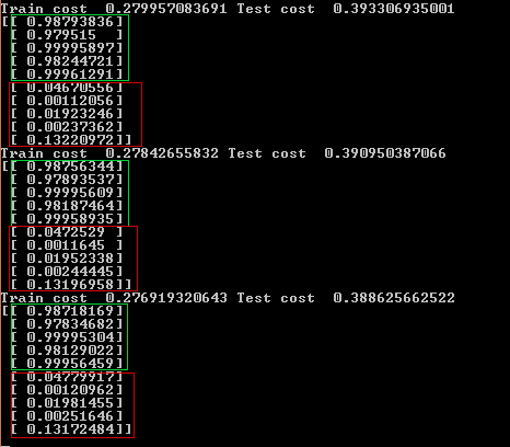
Let's set a simple task, to distinguish an upward trend from a downward one. Neural network input will be fed 4 numbers, if they are consistently increased, this is one, if they decrease, this is zero.
nn=nt.create([4, 1000, 1]) lamb=0.3 cost=1 alf = 0.2 xTrain = [[1, 2.3, 4.5, 5.3], [1.1, 1.3, 2.4, 2.4], [1.9, 1.7, 1.5, 1.3], [2.3, 2.9, 3.3, 4.9], [3, 5.2, 6.1, 8.2], [3.31, 2.9, 2.4, 1.5], [4.9, 5.7, 6.1, 6.3], [4.85, 5.0, 7.2, 8.1], [5.9, 5.3, 4.2, 3.3], [7.7, 5.4, 4.3, 3.9], [6.7, 5.3, 3.2, 1.4], [7.1, 8.6, 9.1, 9.9], [8.5, 7.4, 6.3, 4.1], [9.8, 5.3, 3.1, 2.9]] yTrain = [[1], [1], [0], [1], [1], [0], [1], [1], [0], [0], [0], [1], [0], [0]] xTest= [[0.4, 1.9, 2.5, 3.1], [1.51, 2.0, 2.4, 3.8], [2.6, 5.1, 6.2, 7.2], [3.23, 4.1, 4.3, 4.9], [7.1, 7.6, 8.2, 9.3], [5.78, 5.1, 4.5, 3.55], [6.33, 4.8, 3.4, 2.5], [7.67, 6.45, 5.8, 4.31], [8.22, 6.32, 5.87, 3.59], [9.1, 8.5, 7.7, 6.1]] yTest = [[1], [1], [1], [1], [1], [0], [0], [0], [0], [0]] while cost>0: cost=nt.costTotal(False, nn, xTrain, yTrain, lamb) costTest=nt.costTotal(False, nn, xTest, yTest, lamb) delta=nt.backpropagation(False, nn, xTrain, yTrain, lamb) nn['theta']=[nn['theta'][i]-alf*delta[i] for i in range(0,len(nn['theta']))] print('Train cost ', cost[0,0], 'Test cost ', costTest[0,0]) print(nt.runAll(nn, xTest)) After 400 iterations (about 1 min.) For some reason, the last test case has the highest error (output of the neural network 0.13), most likely in this case it would help to add training data to improve the quality.
In the cycle we change theta in order to achieve the maximum result. It turns out that we are gliding to the local minimum of the function (and if we added a gradient, then we would go to the local maximum). The variable alf, often called the “learning rate”, is responsible for how much we will change theta in each iteration. Moreover, if you set the alpha parameter too large, the network error may even increase or jump up and down as the function will simply step over the local minimum.
As you can see, the entire neural network consists of a single variable of the type dict, so it is easy to make it a secondary one, and save it in a simple text file and also restore it for future use.
Perhaps the next post will be on how to speed up this code (and any other written in Python) using GPU computing.
Full listing of the module, use at your discretion
import copy import numpy as np import random as rd import theano.tensor as th class network: # layers -list [5 10 10 5] - 5 input, 2 hidden # layers (10 neurons each), 5 output def create(self, layers): theta = [0] # for each layer from the first (skip zero layer!) for i in range(1, len(layers)): # create nxM+1 matrix (+bias!) with random floats in range [-1; 1] theta.append( np.mat(np.random.uniform(-1, 1, (layers[i], layers[i - 1] + 1)))) nn = {'theta': theta, 'structure': layers} return nn def runAll(self, nn, X): z = [0] m = len(X) a = [copy.deepcopy(X)] # a[0] is equal to the first input values logFunc = self.logisticFunctionVectorize() # for each layer except the input for i in range(1, len(nn['structure'])): # add bias column to the previous matrix of activation functions a[i - 1] = np.c_[np.ones(m), a[i - 1]] # for all neurons in current layer multiply corresponds neurons z.append(a[i - 1] * nn['theta'][i].T) # in previous layers by the appropriate weights and sum the # productions a.append(logFunc(z[i])) # apply activation function for each value nn['z'] = z nn['a'] = a return a[len(nn['structure']) - 1] def run(self, nn, input): z = [0] a = [] a.append(copy.deepcopy(input)) a[0] = np.matrix(a[0]).T # nx1 vector logFunc = self.logisticFunctionVectorize() for i in range(1, len(nn['structure'])): a[i - 1] = np.vstack(([1], a[i - 1])) z.append(nn['theta'][i] * a[i - 1]) a.append(logFunc(z[i])) nn['z'] = z nn['a'] = a return a[len(nn['structure']) - 1] def logisticFunction(self, x): a = 1 / (1 + np.exp(-x)) if a == 1: a = 0.99999 # make smallest step to the direction of zero elif a == 0: a = 0.00001 # It is possible to use np.nextafter(0, 1) and # make smallest step to the direction of one, but sometimes this step # is too small and other algorithms fail :) return a def logisticFunctionVectorize(self): return np.vectorize(self.logisticFunction) def costTotal(self, theta, nn, X, y, lamb): m = len(X) # following string is for fmin_cg computaton if type(theta) == np.ndarray: nn['theta'] = self.roll(theta, nn['structure']) y = np.matrix(copy.deepcopy(y)) # feed forward to obtain output of neural network hAll = self.runAll(nn, X) cost = self.cost(hAll, y) # apply regularization return cost / m + (lamb / (2 * m)) * self.regul(nn['theta']) def cost(self, h, y): logH = np.log(h) log1H = np.log(1 - h) # transpose y for matrix multiplication cost = -1 * yT * logH - (1 - yT) * log1H # sum matrix of costs for each output neuron and input vector return cost.sum(axis=0).sum(axis=1) def regul(self, theta): reg = 0 thetaLocal = copy.deepcopy(theta) for i in range(1, len(thetaLocal)): # delete bias connection thetaLocal[i] = np.delete(thetaLocal[i], 0, 1) # square the values because they can be negative thetaLocal[i] = np.power(thetaLocal[i], 2) # sum at first rows, than columns reg += thetaLocal[i].sum(axis=0).sum(axis=1) return reg def backpropagation(self, theta, nn, X, y, lamb): layersNumb = len(nn['structure']) thetaDelta = [0] * (layersNumb) m = len(X) # calculate matrix of outpit values for all input vectors X hLoc = copy.deepcopy(self.runAll(nn, X)) yLoc = np.matrix(y) thetaLoc = copy.deepcopy(nn['theta']) derFunct = np.vectorize( lambda x: (1 / (1 + np.exp(-x))) * (1 - (1 / (1 + np.exp(-x))))) zLoc = copy.deepcopy(nn['z']) aLoc = copy.deepcopy(nn['a']) for n in range(0, len(X)): delta = [0] * (layersNumb + 1) # fill list with zeros # calculate delta of error of output layer delta[len(delta) - 1] = (hLoc[n].T - yLoc[n].T) for i in range(layersNumb - 1, 0, -1): # we can not calculate delta[0] because we don't have theta[0] # (and even we don't need it) if i > 1: z = zLoc[i - 1][n] # add one for correct matrix multiplication z = np.c_[[[1]], z] delta[i] = np.multiply( thetaLoc[i].T * delta[i + 1], derFunct(z).T) delta[i] = delta[i][1:] thetaDelta[i] = thetaDelta[i] + delta[i + 1] * aLoc[i - 1][n] for i in range(1, len(thetaDelta)): thetaDelta[i] = thetaDelta[i] / m thetaDelta[i][:, 1:] = thetaDelta[i][:, 1:] + \ thetaLoc[i][:, 1:] * (lamb / m) # regularization if type(theta) == np.ndarray: # to work also with fmin_cg return np.asarray(self.unroll(thetaDelta)).reshape(-1) return thetaDelta # create 1d array form lists like theta def unroll(self, arr): for i in range(0, len(arr)): arr[i] = np.matrix(arr[i]) if i == 0: res = (arr[i]).ravel().T else: res = np.vstack((res, (arr[i]).ravel().T)) res.shape = (1, len(res)) return res # roll back 1d array to list with matrices according to given structure def roll(self, arr, structure): rolled = [arr[0]] shift = 1 for i in range(1, len(structure)): temparr = copy.deepcopy( arr[shift:shift + structure[i] * (structure[i - 1] + 1)]) temparr.shape = (structure[i], structure[i - 1] + 1) rolled.append(np.matrix(temparr)) shift += structure[i] * (structure[i - 1] + 1) return rolled UPD
Thanks to everyone who is a plus.
Source: https://habr.com/ru/post/258611/
All Articles