RMQ Task - 1. Static RMQ
Introduction
The RMQ task is quite common in sports and application programming. It is surprising that on Habré no one has yet mentioned this interesting topic. I'll try to fill the gap.
The abbreviation RMQ stands for Range Minimum (Maximum) Query - a request for the minimum (maximum) on a segment in the array. For definiteness, we will consider the operation of taking a minimum.
')
Let an array A [1..n] be given. We need to be able to respond to the request of the form "to find the minimum in the segment from the i-th element to the j-th one".
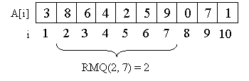
Consider as an example the array A = {3, 8, 6, 4, 2, 5, 9, 0, 7, 1}.
For example, the minimum on the segment from the second element to the seventh is equal to two, that is, RMQ (2, 7) = 2.
The obvious solution comes to mind: we will find the answer to each request, simply by running over all the elements of the array lying on the segment we need. Such a solution, however, is not the most effective. Indeed, in the worst case, we will have to run through O (n) elements, i.e. The time complexity of this algorithm is O (n) per request. However, the problem can be solved more effectively.
Formulation of the problem
First, let's clarify the problem statement.
What does the word static mean in the title of the article? The RMQ task is sometimes set with the ability to change the elements of an array. That is, the possibility of changing an element, or even changing elements on a segment (for example, increasing all elements on a sub-segment by 3), is added to the minimum request. This version of the task, called dynamic RMQ, I will look at in subsequent articles.
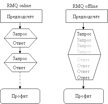
I note here that the RMQ task is divided into offline and online versions. In an offline version, you can first receive all requests, analyze them in some way and only then give an answer to them. In the online -statement, requests are given in turn, i.e. The next request comes only after a response to the previous one. Note that by solving RMQ in an online -statement, we immediately get a solution for offline RMQ, although there may be a more efficient solution for offline RMQ, which is not applicable for online -setting.
In this article, we will look at static online RMQ.
Preprocessing time
To assess the efficiency of the algorithm, we introduce another time characteristic — the preprocessing time. We will take into account the preparation time, i.e. Pre-account some information needed to respond to requests.
It would seem, why do we need to allocate preprocessing separately? But why? We give another solution to the problem.
Before you begin to respond to requests, take and just count the answer for each segment! Those. we will construct an array of P [n] [n] (in the following I will use a C-like syntax, although array A will be numbered from one for ease of implementation), where P [i] [j] will be equal to the minimum on the segment from i to j. And we will count this array even for O (n 3 ) - in the most stupid way, running over all the elements for each segment. Why do we do this? Suppose the number of queries q is much more than n 3 . Then the total running time of our algorithm is O (n 3 ) + q * O (1) = O (q), i.e. The preprocessing time is by and large and will not affect the total running time of the algorithm. But thanks to the compiled information, we learned how to respond to a request in O (1) time instead of O (n). It is clear that O (q) is better than O (qn).
On the other hand, when q <n 3 , the preprocessing time will play its role, and in the above algorithm it is O (n 3 ), unfortunately, is too long, even though it can be reduced (think how) to O (n 2 ).
From this point on, we will denote the time characteristics of the algorithm as (P (n), Q (n)), where P (n) is the time for the pre-count and Q (n) is the time to respond to one request.
So, we have two algorithms. One works for (O (1), O (n)), the second for (O (n 2 ), O (1)). Let's learn how to solve the problem in (O (nlogn), O (1)), where logn is the binary logarithm of n.
Lyrical digression. Note that you can take any number as the base of the logarithm, since log a n always differs from log b n exactly a constant number of times. The constant, as we remember from the course of school algebra, is equal to log a b.
So, we have reached the next step:
Sparse Table, or Sparse Table
Sparse Table is a table ST [] [] such that ST [k] [i] is the minimum in the half-interval [A [i], A [i + 2 k ]). In other words, it contains minima on all segments whose length is a power of two.
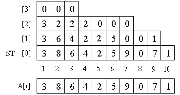
We calculate the array ST [k] [i] as follows. It is clear that ST [0] is simply our array A. Then we use the clear property:
ST [k] [i] = min (ST [k-1] [i], ST [k-1] [i + 2 k - 1 ]). Thanks to him, we can first calculate ST [1], then ST [2], and so on.
Note that in our table O (nlogn) elements, because the level numbers must be no more than logn, since for large values of k the length of the half-interval becomes longer than the length of the entire array and storing the corresponding values is meaningless. And at every level of O (n) elements.
Lyrical digression again: It is easy to see that we still have a lot of unused elements of the array. Shouldn't a table be stored differently in order not to waste memory? Let us estimate the amount of unused memory in our implementation. On the i-th row of unused elements - 2 i - 1. Hence, the total unused remains Σ (2 i - 1) = O (2 logn ) = O (n), i.e. in any case, you will need about O (nlogn) - O (n) = O (nlogn) storage space for the Sparse Table. So you can not worry about unused items.
And now the main question: why did we think all this? Note that any segment of the array is divided into two overlapping subsegments of a power of two.

We obtain a simple formula for calculating RMQ (i, j). If k = log (j - i + 1), then RMQ (i, j) = min (ST (i, k), ST (j - 2 k + 1, k)). Thus, we get the algorithm for (O (nlogn), O (1)). Hooray!
... almost get it. How do we log the logarithm gathered for O (1)? The easiest way is also to presuppose it for all values not exceeding n. It is clear that the asymptotics of the preprocessing will not change.
What's next?
And in subsequent articles we will look at the many variations of this task and the plots associated with them, such as:
- segment tree
- interval modification
- two-dimensional segment tree
- related RSQ task
- Fenwick tree
- LCA task
- RMQ persistent task setting
- ... a lot of interesting things ...
- and the beauty: the Farah-Colton and Bender algorithm and the transformation RMQ -> LCA -> RMQ ± 1, which allows to solve the problem RMQ for (O (n), O (1))
For details, you can refer, for example, to the smart book by T. Kormen, C. Leiserson, and R. Rivest “Algorithms: construction and analysis”.
Other topics will appear in subsequent topics.
Thank you for attention.
Source: https://habr.com/ru/post/114980/
All Articles