Darts, dice and coins: discrete sampling algorithms

Once I asked on Stack Overflow a question about the data structure for the cheating dice . In particular, I was interested in the answer to this question: “If we have an n-sided bone, the face of which i has the probability of falling out p i . What is the most efficient data structure for simulating such a dice? ”
This data structure can be used for many tasks. For example, you can use it to simulate the throws of an honest hex bone, assigning the probability f r a c 1 6 each side of the bone, or to simulate an honest coin by imitating a double-sided bone, the probability of each side falling out is f r a c 1 2 . You can also use this data structure to directly simulate the sum of two honest hexagonal bones by creating an 11-sided bone (with faces of 2, 3, 4, ..., 12), each face of which has a probability weight corresponding to the rolls of two honest bones. However, you can also use this data structure to simulate cheat bones. For example, if you play craps with a bone that you know is not perfectly fair, then you can use this data structure to simulate a variety of bone rolls and analyze the optimal strategy. You can also try to simulate a similarly imperfect roulette wheel .
If you go beyond the limits of the games, you can apply this data structure in the simulation of robots, the sensors of which have known levels of failure. For example, if the range sensor has a 95 percent probability of returning the correct value, a 4 percent probability of too small a value, and a 1 percent probability of a too large value, then you can use this data structure to simulate the reading of the sensor by generating a random result and simulating the reading of the sensor result.
The response I received at Stack Overflow impressed me for two reasons. First, in the decision I was advised to use a powerful technique called the alias-method , which, with certain reasonable assumptions about the model of the machine, is capable, after a simple preliminary preparation stage, to simulate rolls of the dice during O ( 1 ) . Secondly, I was even more surprised by the fact that this algorithm has been known for decades, but I have never met it! Given how much computational time is spent on the simulation, one would expect that this technique is known much more widely. Several queries to Google gave me a lot of information about this technique, but I could not find a single site where the intuitive understanding and explanation of this technique would be connected.
')
This article is my attempt to make a brief overview of various approaches to the simulation of a cheat bone, from simple and very impractical techniques, to a very optimized and effective alias method. I hope that I will be able to convey the different ways of the intuitive understanding of the task and the extent to which each of them emphasizes some new aspect of the simulation of the cheat bone. My goal for each approach is to study the motivating idea, the basic algorithm, proof of correctness and analysis of the execution time (in terms of the required time, memory and randomness).
Introduction
Before proceeding to the specific details of various techniques, let's first standardize the terminology and notation.
In the introduction to the article, I used the term “cheat bone” to describe a generalized scenario in which there is a finite set of results, each of which has a probability, Formally, this is called a discrete probability distribution , and the task of simulating a cheat bone is called a sample from a discrete distribution .
To describe our discrete probability distribution (shuler's bone), we will assume that we have a set of n probabilities p 0 , p 1 , . . . , p n - 1 related to results 0 , 1 , . . . , n - 1 . Although the results can be any (eagle / tails, numbers on bones, colors, etc.), for simplicity, I will consider the result to be some positive real number corresponding to a given index.
Working with real numbers on a computer is a “gray area” of computing. There are many fast algorithms whose speed is provided solely by the ability to calculate the floor function of an arbitrary real number in constant time, and numerical inaccuracies in the representation of floating-point numbers can completely destroy some algorithms. Therefore, before embarking on any discussion of algorithms that work with probabilities, that is, to enter into the dark world of real numbers, I must clarify what a computer can and cannot do.
Hereinafter, I will assume that all of the following operations can be performed in constant time:
- Addition. subtraction, multiplication, division and comparison of arbitrary real numbers . We will need to do this to manipulate probabilities. It may seem that this is too bold an assumption, but if we assume that the accuracy of any real number is limited by a certain word-size polynomial of the machine (for example, 64-bit double on a 32-bit machine), but I do not think that this is too unreasonable.
- Generation of a uniform real number in the interval [0, 1). To simulate randomness, we need some source of random values. I assume that we can generate a real number of arbitrary precision in constant time. This far exceeds the capabilities of a real computer, but it seems to me that this is acceptable for the purposes of this discussion. If we agree to sacrifice a bit of precision, saying that an arbitrary IEEE-754 double is in the interval [0, 1], then we really lose accuracy, but the result is likely to be accurate enough for most applications.
- Calculating the integer floor (rounding down) of a real number. This is permissible if we assume that we are working with IEEE-754 double, but in general, such a requirement for a computer is impracticable.
It is worth asking whether it is reasonable to assume that we can perform all these operations efficiently. In practice, we rarely use the probabilities specified to such a level of accuracy at which the inherent IEEE-754 double rounding error can cause serious problems, so we can fulfill all the above requirements simply by working exclusively with IEEE double. However, if we are in an environment where probabilities are indicated exactly as rational numbers of high accuracy, then such restrictions may turn out to be unreasonable.
Simulation of honest bones
Before we move on to the more general case of throwing an arbitrary cheat bone, let's start with a simpler algorithm that serves as a building block for subsequent algorithms: with a simulation of an honest n-face bone. For example, throws of an honest 6-faced dice can be useful to us when playing Monopoly or Risk, or throwing an honest coin (double-sided dice), etc.
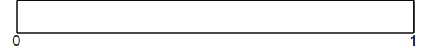
For this particular case, there is a simple, elegant, and efficient algorithm for simulating the result. The algorithm is based on the following idea: Suppose that we can generate really random, uniformly distributed real numbers in the interval [ 0 , 1 ) . To illustrate this interval as follows:
Now if we want to quit n -cut bone, one of the ways is to divide the interval [ 0 , 1 ) on n areas of equal size, each of which has a length f r a c 1 n . It looks like this:
Next, we generate a randomly selected real number in the interval [ 0 , 1 ) which exactly fits into one of these small areas. From this we can count the result of the roll of the dice, looking at the area in which the number fell. For example, if our randomly chosen value fell into this place:

then we can say that the bone has fallen 2 (if we assume that the edges of the bone are indexed from scratch).
It is graphically easy to see which of the regions got a random value, but how do we encode it in the algorithm? And here we take advantage of the fact that this is an honest bone. Since all intervals are of equal size, namely f r a c 1 n then we can see which is the greatest value i is such that f r a c i n no more randomly generated value (let's call this x value). You may notice that if we want to find the maximum value, such that fracin lex then this is similar to finding the maximum value n such that i lexn . But this by definition means that i= lfloorxn rfloor , the greatest positive integer is not greater than xn. Therefore, this leads us to the following (very simple) algorithm for simulating an honest n-face bone:
Algorithm: honest bone simulation
- We generate a uniformly distributed random value. x in the interval [0,1) .
- Return lfloorxn rfloor .
Given our computational assumptions made above, this algorithm runs in time. O(1) .
Two conclusions can be drawn from this section. First, we can divide the interval [0,1) into parts so that a uniformly distributed random real number in this interval naturally reduces to one of the many discrete choices available to us. In the rest of the article we will actively exploit this technique. Secondly, it can be difficult to determine which specific interval a random value belongs to, but if we know something about the parts (in this case, that they are all the same size), then it can be mathematically simple to determine which part exactly point.
Simulation of a cheat bone using honest bone
Having an honest bone simulation algorithm, can we adapt it to simulate a cheat bone? Interestingly, the answer is yes, but the solution will require more space.
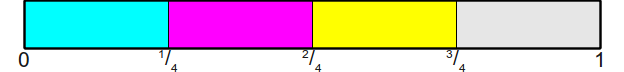
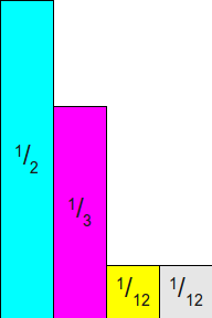
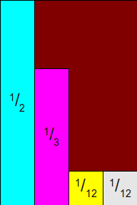
From the previous section, it is intuitively clear that in order to simulate the throw of a cheat bone, it suffices to divide the interval [0,1) into parts, and then determine which part we hit. However, in general, this may be much more complicated than it seems. Suppose we have a tetrahedral bone with face probabilities frac12 , frac13 , frac112 and frac112 (we can make sure that this is the correct probability distribution, because frac12+ frac13+ frac112+ frac112= frac612+ frac412+ frac112+ frac112= frac1212 ). If we divide the interval [0,1) into four pieces of these sizes, we get the following:

Unfortunately, at this step we will be stuck. Even if we knew a random number in the interval [0,1) then there are no simple mathematical tricks to automatically determine which part of this number fell into. I do not want to say that this is impossible - as you will see, we can use many excellent tricks - but none of them has the mathematical simplicity of an honest bone throw algorithm.
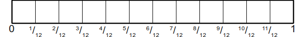
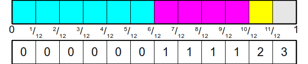
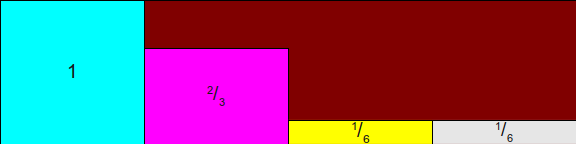
However, we can adapt the technique used for honest bones so that it works in this case as well. Let's take, for example, the bone discussed above. The probability of falling faces is equal to frac12 , frac13 , frac112 and frac112 . If we rewrite it so that all members have a common divisor, we get the values frac612 , frac412 , frac112 and frac112 . Therefore, we can perceive this task as follows: instead of throwing a tetrahedral bone with weighted probabilities, why not throw a 12-sided honest bone, on the edges of which there are repetitive values? Since we know how to simulate honest bone, this will be analogous to dividing the interval [0,1) on the part in this way:
Then we assign them to various results as follows:
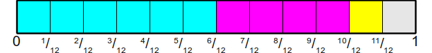
Now, it will be very easy to simulate a roll of the dice - we just throw this new honest bone, and then we look at which side fell out and read its value. This first step can be performed by the above algorithm, which will give us an integer number in the interval 0,1,...,11 . To bind this integer to one of the faces of the original cheat bone, we will store an auxiliary array of twelve elements, connecting each of these numbers with the original result. Graphically, this can be represented as:
In order to formalize this in the form of an algorithm, we will describe both the initialization stage (obtaining the table) and the generation stage (simulation of a random bone roll). Both of these steps are important to consider in this and subsequent algorithms, because the preparation time should be excellent.
At the initialization stage, we begin with the search for the smallest common multiple of all the probabilities specified for the edges of the bone (in our example, the LCM is 12). The NOC is useful here because it corresponds to the smallest common divisor that we can use for all fractions, and therefore the number of faces of the new honest dice that we will throw. Having received this LCM (we denote it L), we must determine how many faces of the new bone will be distributed on each of the faces of the original cheat bone. In our example, the edge with probability frac12 gets six sides of a new bone since frac12 times12=6 . Similarly, the side with the probability frac13 gets 4 faces since frac13 times12=4 . In a more generalized form, if L is the NOK of probabilities, and pi is the probability of falling face i bones then we will highlight the faces i original cheat bone L cdotpi facets of honest bone.
Here is the pseudocode of the above algorithm:
Algorithm: simulation of a cheat bone using honest bone
- Initialization :
- Find the NOK denominators of probabilities p0,p1,...,pn−1 ; denote it L
- Select the array A size L for comparing the results of throwing an honest bone with the throws of the original bone.
- For each face i source bone perform in any order the following:
- We assign the following L cdotpi elements A value i .
- Generation :
- We generate a roll of honest bones for L - bone; call the face S .
- Return A[s] .
Perhaps this algorithm is simple, but how effective is it? The very generation of throwing the dice is fast enough - each throw of the dice requires O(1) work time to generate a random roll of the dice using the previous algorithm, plus another O(1) work time on the search table. This gives us a total work time. O(1) .
However, the initialization step can be extremely expensive. To make this algorithm work, we need to allocate space for an array the size of the LCM denominators of all input fractions. In our example ( frac12 , frac13 , frac112 , frac112 ), it is equal to 12, for with other input values, the values may be pathologically bad. For example, let's consider fractions frac9999991,000,000 and frac11000000 . The LCM denominators are equal to one million, therefore there should be one million elements in our table!
Unfortunately, things can be even worse. In the previous example, we can at least “expect” that the algorithm will take a lot of memory, since both denominators of fractions are equal to one million. However, we may have a lot of probabilities for which the NOC is much larger than each individual denominator. For an example, let's look at probabilities. frac115 , frac110 , frac56 . Here the NOC denominators are 30, which is more than any of the denominators. The design works here because 15=3 times5 , 10=2 times5 , but 6=2 times3 ; in other words, each denominator is a product of two primes selected from a pool of three values. Therefore, their LCM is the product of all these primes, since each denominator must be a divisor of LCM. If we generalize this construction and consider any set of k primes and take one fraction for each of the pairwise products of these primes, the LCM will be much larger than each individual denominator. In fact, one of the best upper bounds we can get for an NOC will be O( prodni=0di) where di - this is the denominator i -This probability. This does not allow the use of such an algorithm in real conditions, when the probabilities are unknown in advance, since the memory required to store the size table O( prodni=0di) , can easily be more volume that can fit in RAM.
In other words, in many cases this algorithm behaves well. If all probabilities are the same, then all probabilities obtained at the input are equal frac1n for some n . Then the LCM denominators are n that is, as a result, an honest bone being thrown will have n faces, and each face of the original bone will correspond to one facet of honest bone. Therefore, the initialization time is O(n) . Graphically, this can be represented as:
This gives us the following information about the algorithm:
| Algorithm | Initialization time | Generation time | Occupied memory | |||
|---|---|---|---|---|---|---|
| The best | Worst | The best | Worst | The best | Worst | |
| Honest bone cheat bone | Theta(n) | O( prodni=0di) | Theta(1) | Theta(n) | O( prodni=0di) | |
Another important detail about this algorithm: it assumes that we will get convenient probabilities in the form of fractions with good denominators. If the probabilities are set as IEEE-754 double, then this approach is most likely waiting for a catastrophe because of small rounding errors; Imagine that we have probabilities of 0.25 and 0.250000000001! Therefore, it is probably better not to use such an approach, except for special cases when the probabilities behave well and are indicated in a format corresponding to operations with rational numbers.
Simulation Asymmetric Coin
Our explanation of a simple random primitive (honest bone) led to a simple, but potentially terribly inefficient algorithm for simulating a cheat bone. Perhaps the study of other simple random primitives will shed some light on other approaches to solving this problem.
A simple but surprisingly useful task is to simulate an asymmetric coin using a random number generator. If we have a coin with the probability of falling eagle pheads , how can we simulate the throw of such an asymmetric coin?
Earlier, we developed one intuitive approach: splitting the interval [0,1) on the sequence of such areas that, when choosing a random value in the interval, it turns out to be in some area with a probability equal to the size of the area. To simulate an asymmetric coin using a uniformly distributed random value in the interval [0,1) we have to split the interval [0,1) in the following way:

And then generate a uniformly distributed random value in the interval [0,1) to see in which area it is contained. Fortunately, we have only one split point, so it is very easy to determine in which area the point is located; if the value is less pheads then the eagle fell on the coin, otherwise tails. Pseudocode:
Algorithm: Asymmetric Coin Simulation
- We generate a uniformly distributed random value in the interval. [0,1) .
- If a x<pheads , return the "eagle".
- If a x gepheads , return "tails."
Since we can generate a uniformly distributed random value in the interval [0,1) during O(1) and we can also make a comparison of real numbers for O(1) then this algorithm runs in time O(1) .
Honest bone simulation using asymmetrical coins
From the previous discussion, we know that you can simulate a cheat bone with the help of an honest bone, if we assume that we are ready to spend extra space in memory. Since we can perceive an asymmetric coin as a cheating two-sided bone, this means that we can simulate an asymmetric coin with the help of an honest bone. Interestingly, the opposite can be done - to simulate an honest bone with the help of an asymmetric coin. The design is simple, elegant, and can be easily generalized to simulate a cheat bone using a variety of asymmetric coins.
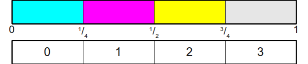
The design for simulating an asymmetric coin breaks the spacing [0,1) on two areas - the area of "eagles" and the area of "tails" based on the probability of eagles falling on the bones. We have already seen a similar trick used to simulate an honest n - face bone: spacing [0,1) divided into n equal areas. For example, when throwing a tetrahedral bone, we had the following separation:
Now suppose that we are interested in simulating the throw of this honest bone using a set of asymmetric coins. One solution is as follows: Imagine that we are going around these areas from left to right, asking each time if we want to stop in the current area, or we will move on. For example, let's assume that we want to randomly select one of these areas. Starting from the leftmost area, we will flip an asymmetrical coin that tells us whether we should stop in this area or continue on. Since we need to choose from all these areas evenly with probability frac14 , then we can do this by throwing an asymmetrical coin, the eagles on which fall out with probability frac14 . If an eagle falls, then we stop in the current area. Otherwise we move to the next area.
If coins fall flat up, then we find ourselves in the second area and again ask if we should again select this area or continue moving. You might think that for this we need to throw another coin with the probability of a falling eagle frac14 but in fact this is not true! To see a flaw in this reasoning, we have to go to an extreme situation - if in each area we throw a coin, on which an eagle falls, with probability frac14 , that is, there is a small probability that in each area the coin will fall out of the tail, that is, we will have to abandon all areas. When moving through the regions, we somehow need to continue to increase the likelihood of an eagle falling on a coin. In an extreme situation, if we are in the last area, then the coin must have an eagle with a probability 1 because if we rejected all previous areas, then the correct solution would be to stop at the last area.
In order to determine the probability with which our asymmetrical coin must eject an eagle after the first region is skipped, we need to note that after the first region skips, there are only three of them left. As we roll honest bone, we need each of these three areas to be selected with probability frac13 . Therefore, it seems intuitively that we should have a second bone, on which an eagle falls on frac13 . Using similar reasoning, it can be understood that when a tails out in the third region in the third region, the coin should fall out with an eagle with probability frac12 , and in the latter area - with probability 1 .
Such an intuitive understanding leads us to the following algorithm. Note that we did not discuss the correctness or error of this algorithm; Soon we will do it.
Algorithm: simulation of honest bone using asymmetric coins
- For i=0 to n−1 :
- Throw asymmetrical coin with the probability of ejection frac1n−i .
- If the eagle falls, then return i .
This algorithm is simple and in the worst case it is executed in time. O(n) . But how do we check if it is correct? To find out, we need the following theorem:
Theorem: the above algorithm returns the side i with probability frac1n for any selected i .
Proof: consider any constant n ge0 . We prove by strong induction that each of n faces has a probability of choice frac1n .
For our example, we show that the face 0 bones have a chance of choosing frac1n . But it directly follows from the algorithm itself - we choose the face 0, if on an asymmetric coin with the probability of falling out of an eagle frac1n an eagle falls, that is, we chose it with probability frac1n .
For the induction phase, assume for the faces 0,1,2,...,k−1 that these edges are chosen with probability frac1n and consider the probability of choosing a face k . The brink k will be selected if and only if not selected first k faces, and on the coin with the probability of falling eagle frac1n−k fell eagle. Since each of the first k faces has a probability of choice frac1n , and since only one face is selected, the probability of choosing one of the first faces k set as frackn . This means that the probability that the algorithm does not choose one of the first k faces equals 1− frackn= fracnn− frackn= fracn−kn . That is, the probability of choosing a face k set as fracn−kn frac1n−k= frac1n what is required to show. Thus, each face of the bone is selected evenly and randomly.
Of course, the algorithm is rather inefficient - with the help of the first technique, we can simulate a throw of an honest bone in time. O(1) ! But this algorithm can be used as a stepping stone to a fairly efficient algorithm for simulating a cheat bone using asymmetric coins.
Simulation of the cheat bone using asymmetric coins
The above algorithm is interesting because it gives us a simple framework for simulating a bone using a set of coins. We start by throwing a coin to determine whether to choose the first face of the dice or move to the remaining ones. In this process, we need to carefully handle the rescaling of the remaining probabilities.
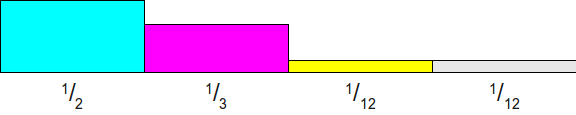
Let's see how this technique can be used to simulate the throw of a cheat bone. Let's use our example with probabilities. frac12 , frac13 , frac112 , frac112 . He, if you do not remember, divides the interval [0,1) in the following way:
Now let's think about how you can simulate such a cheat bone using asymmetric coins. We can start by throwing a coin with the probability of a falling eagle. frac12 to determine whether we should return the verge 0. If an eagle falls on this coin, then great! We are done. Otherwise, we need to throw another coin to decide whether to choose the next facet. As before, despite the fact that the next facet has the probability of choosing frac13 we do not want to throw a coin on which the eagle falls with probability frac13 because half of the “mass” of probabilities was dropped when we did not choose the line with frac12 . In fact, since half of the mass of probabilities has disappeared, then if we normalize the remaining probabilities anew, we will get updated probabilities: frac23 , frac16 , frac16 . Consequently, the second coin must be thrown with probability frac23 . If this coin also falls out of the tail, we will have to choose between the two sides. frac112 . Since at this stage we will get rid of frac56 probability masses, then we can normalize the probabilities of the sides frac112 so that each had a chance frac12 the falling of the eagle, that is, the third coin will have the probability frac12 . The last coin, if it ever comes down to it, should throw out the eagle with probability 1 since this is the latest area.
To summarize, the probabilities of the coins will be as follows:
- First shot: frac12
- Second shot: frac23
- The third shot: frac12
- Fourth Shot: 1
It may be intuitively clear where these numbers come from, but in order to turn selection into an algorithm, we will have to create a formal construction of the choice of probabilities. The idea will be as follows - at each stage we remember the rest of the mass of probabilities. In the beginning, before the roll of the first coin, it is equal to 1 . After throwing the first coin 1−p0 . After throwing the second coin 1−p0−p1 . More generally after the throw k the remaining mass of the probability is 1− sumk−1i=0pi . Every time we throw a coin to determine whether or not to choose a region k , we as a result throw a coin, the probability of falling of an eagle on which is equal to the fraction of the remaining probability occupied by the probability pk what is given as fracpk1− sumk−1i=0pi . This gives us the following algorithm for simulating a cheat bone with a set of asymmetric coins (we will prove its correctness and execution time just below):
Algorithm: cheat bone from asymmetric coins
- Initialization :
- Save probabilities pi for future use.
- Generation :
Ask mass=1
For i=0 to n−1 :
- We throw an asymmetrical coin with the probability of a falling eagle fracpimass .
- If the eagle fell, then return i .
- Otherwise, ask mass=mass−pi
From an intuitive point of view, this is logical, but is it true mathematically? Fortunately, the answer is positive due to the generalization of the above proof:
Theorem: the algorithm shown above returns the face i with probability pi for any chosen i .
Proof: consider any constant n ge0 . With strong induction, we prove that each of n faces has a probability of choice pi .
As a base case, we prove that the face 0 bones have a chance of choosing p0 . We choose the face 0 , if at the roll of the very first coin we get an eagle, what happens with the probability p0mass . mass 1 , p01=p0 , 0 p0 , .
, 0,1,...,k−1 p0,p1,...,pk−1 k . k , k , pkmass . k , , k ∑k−1i=0pi . , k 1−∑k−1i=0pi . , k , pkmass k , mass=1−∑k−1i=0pi . , k ( 1 - ∑ k - 1 i = 0 p i ) p k1 - ∑ k - 1 i = 0 p i =pk, as required.
Now let's estimate the time complexity of this algorithm. We know that the initialization time can beΘ ( 1 ) if we save a surface copy of the input probability array, but it may beΘ ( n ) so that we can save our own version of the array (in case the calling function wants to change it later). The very generation of the result of throwing the dice may require at worstΘ ( n ) throws, and only one throw at best.
However, after thinking it becomes clear that the number of required coin tosses is strongly influenced by the incoming distribution. In the best case, we will have a probability distribution, in which the entire mass of probabilities is concentrated on the first face of the bone, and all other probabilities are zero. In this case, one throw of a coin is enough for us. In the worst case, the entire probability mass is concentrated at the very last face of the bone, and is zero on all other faces. In this case, we will have to throw to get the result.n coins.
We can clearly and mathematically characterize the expected number of coin flips in this algorithm. Let's imagine a random variableX , denoting the number of coin flips for any execution of this algorithm for a particular distribution. I.e P [ X = 1 ] is the probability that to complete the algorithm it is enough to throw one coin,P [ X = 2 ] - the probability that the algorithm will throw two coins, etc. In this case, the expected number of coin flips for our algorithm is determined by theexpectation X , denoted asE [ X ] . By definition, we get that
E [ X ] = n Σ i = 1 i ⋅ P [ X = i ]
What is the meaning P [ X = i ] ?The algorithm terminates after selecting a facet of a bone. If he chooses a face0 , then throw one coin. If he chooses a face1 , then will throw two coins - one to understand that he does not want to choose the face0 , another to understand that he wants to choose the faceone . If more generally, then if the algorithm chooses a face i will throwi + 1 coins:i coins to decide he doesn't want to pick previous onesi - 1 facet, and one to decide what face to choosei . Combined with the fact that we know about choosing a face i with probabilityp i , it means that
E[X]=n∑i=1i⋅P[X=i]=n∑i=1i⋅pi−1=n∑i=1((i−1)pi−1+pi−1)=n∑i=1((i- 1 ) p i - 1 ) + n ∑ i = 1 p i - 1
Note that in the last simplification, the first term is equivalent to ∑ n - 1 i = 0 i ⋅ p i , which is equivalentE [ p ] , the expected outcome of a dice roll! Moreover, the second term is1 , since this is the sum of all probabilities. It means thatE [ X ] = E [ p ] + 1 . That is, the expected number of throws of coins is equal to one plus the expected expectation of a dice roll!
| Algorithm | Initialization time | Generation time | Busy memory | |||
|---|---|---|---|---|---|---|
| The best | Worst | The best | Worst | The best | Worst | |
| Honest bone cheat bone | Θ ( n ) | O ( ∏ n i = 0 d i ) | Θ ( 1 ) | Θ ( n ) | O ( ∏ n i = 0 d i ) | |
| Shuler bone from asymmetrical coins | Θ ( n ) | Θ ( 1 ) | Θ ( n ) | Θ ( n ) | ||
Generalization of asymmetrical coins: simulation of a cheat bone
In the example shown above, we were able to effectively simulate an asymmetric coin, since we only had to take into account one split point. How can we effectively generalize this idea to a cheat bone, in which the number of faces can be arbitrary?
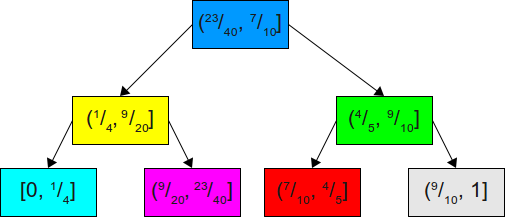
As you can see, an asymmetric coin is a cheat bone, with only two faces. Consequently, we can perceive an asymmetric coin simply as a special case of a more general problem that we want to solve. In solving the problem of an asymmetric coin, we divide the interval[ 0 , 1 ) into two areas - one for the eagle, the second for tails - and then to find the area we use the fact that there is only one splitting point. If we have an n-sided bone, then there will be more areas, and therefore several dividing points. Suppose, for example, that we have a seven-sided bone with probabilitiesonefour , onefive , oneeight , oneeight , oneten , oneten , oneten . If we want to divide the interval [ 0 , 1 ) into seven parts, then do it as follows:
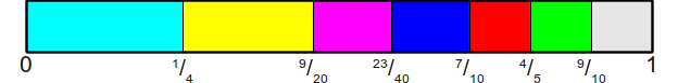
Notice where these areas are located. The first area starts with0 and endsonefour . The second area begins with one4 and ends atone4 +15 =920 . More generally, if the probabilities are equal p 0 , p 1 , . . . , p n - 1 , then the regions will be intervals[ 0 , p 0 ) , [ p 0 , p 0 + p 1 ) , [ p 0 + p 1 , p 0 + p 1 + p 2 ) etc. That is the area i is limited by the interval
[ i - 1 ∑ j = 0 p j , i ∑ j = 0 p j )
Notice that the difference between these two values is p i , that is, the total area of the region is equal top i , as required.
Now we know where the regions are. If we want to choose a uniformly distributed random valuex in the interval[ 0 , 1 ) , then how do we determine at what interval it falls? If we use our asymmetric coin algorithm as a starting point, the idea will be as follows: starting from the end point of the first area, constantly move upwards through all areas until we find the end point whose value is greater thanx . If we do this, we will find the first area containing the point x , which means our value. For example, if we selected a random valuex = 2740 , then perform the following search:
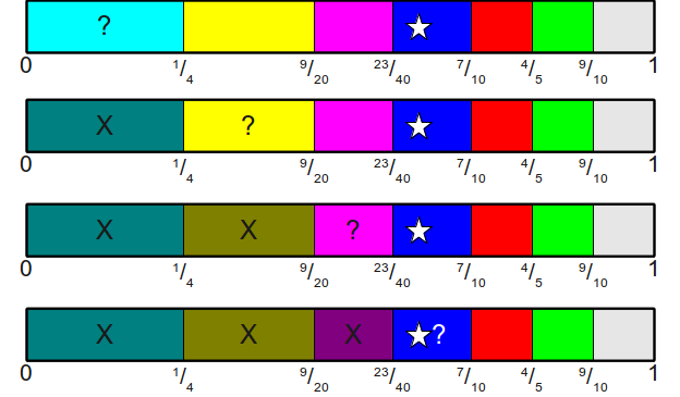
From what we can conclude that the edge 3 fell on the bone indexed from scratch.
Such a linear scanning algorithm will give us an algorithm of timeO ( n ) to find the discarded face of the bone. However, we can significantly improve its execution time using the following observation: a series of endpoints of regions form an increasing sequence (since we always add more and more probabilities, none of which can be less than zero). Therefore, we want to answer the following question: having an increasing sequence of values and a certain check point, we need to find the first value in the interval that is strictly greater than the check point. This is the perfect moment to usebinary search! For example, here's a binary search on the above array to find the area to whichx = 3940 :

This gives us an algorithm with time. Θ ( log n ) to bind a uniformly distributed random value in the interval[ 0 , 1 ) to the verge of an abandoned bone. Moreover, there is enough preprocessing time to build the endpoint table.Θ ( n ) ;we simply calculate partial sums of probabilities as we move up.
This algorithm is sometimes called the roulette wheel selection algorithm , because it selects a random area using a roulette wheel-like technique — throwing the ball at intervals and observing where it stops. In pseudocode, the algorithm looks like this:
Algorithm: selection by the roulette wheel
- Initialization :
- Select the array A size n
- Ask A [ 0 ] = p 0 .
- For each probability i from one before n - 1 :
- Ask A [ i ] = A [ i - 1 ] + p i
- Generation :
- We generate a uniformly distributed random value. x in the interval[ 0 , 1 )
- Using binary search we find the index i of the smallest elementA which is lessx .
- Return i .
The comparison between this algorithm and the one mentioned earlier looks quite impressive:
| Algorithm | Initialization time | Generation time | Busy memory | |||
|---|---|---|---|---|---|---|
| The best | Worst | The best | Worst | The best | Worst | |
| Honest bone cheat bone | Θ(n) | O(∏ni=0di) | Θ(1) | Θ(n) | O(∏ni=0di) | |
| Θ(n) | Θ(1) | Θ(n) | Θ(n) | |||
| Θ(n) | Θ(logn) | Θ(n) | ||||
Obviously, now we have a much better algorithm than the original one. Discretization of probabilities only seemed promising at first, but this new approach based on continuous value and binary search looks much better. However, it is still possible to improve these indicators through the clever use of a set of hybrid techniques that we will discuss below.
An interesting detail of this algorithm is that although the use of a binary search ensures the worst time for generating random numbersO ( log n ) , it also does not allow a faster search; that is, the generation time will also be equalΩ ( log n ) .Can it be improved? It turns out that you can.
Suppose we move from a binary search through a list of accumulated probabilities to using a binary search tree . For example, having the above set of probabilities, we can build the following binary search tree for their accumulated distribution:
Now, if we want to simulate a dice roll, we can generate a uniformly distributed number in the interval. [ 0 , 1 ) , and then see in what interval it lies in this binary search tree (BST). Since this is a balanced binary search tree, the best search time isO ( 1 ) , and the worst -O ( log n ) .
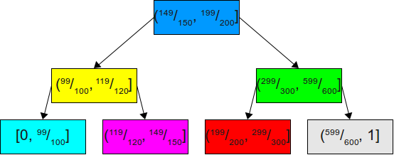
However, if we assume that we know more about the probability distribution, then we can do much better. For example, suppose our probabilities are equal99100 , one600 , one600 , one600 , one600 , one600 , one600 .That is, the probability distribution is extremely skewed, and almost the entire mass of probabilities is concentrated on one face. We can build a balanced BST for these probabilities:
Although this binary search tree is perfectly balanced, it is not very suitable for our tasks. Since we know that in 99 out of 100 cases a random value will be in the range[ 0 , 99100 ), then there is no point in keeping the node for this interval where it is located now. In fact, this will mean that almost all the time we will be performing two unnecessary comparisons with the blue and yellow areas. Since, with a very high probability, we should first check the largest interval, it would be logical to unbalance the tree so as to make the average case much better at the expense of the rest. This is shown here:
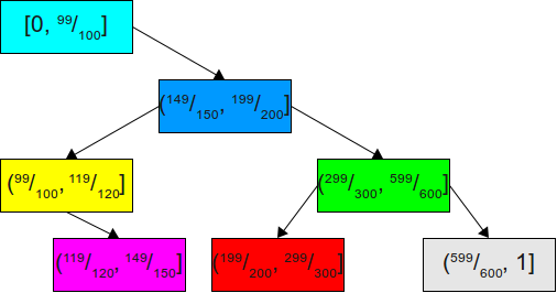
Now we are likely to complete the search, immediately finding the desired area after the first attempt. In the very unlikely event that the desired area is in the remaining( 99100 ,1]we will quietly descend to the end of the tree, which is actually well balanced.
In a generalized form, we want to solve the following problem:
Given a given set of probabilities, find the binary search tree of these probabilities, which minimizes the expected search time.
Fortunately, this problem is very well studied and is called the optimal binary search tree problem . There are many algorithms to solve this problem; It is known that the exact solution can be found in time. O ( n 2 ) using dynamic programming , and that there are good linear time algorithms that can find approximate solutions. In addition, the splay tree data structure (expanding tree) (self-balancing binary search tree) can be used to obtain a constant multiplier for the optimal solution.
It is interesting that the best case behavior of such optimized binary search trees occurs when probability distributions are extremely skewed, since we can simply move nodes containing the vast majority of probabilities to the root of the tree, and the worst case is when the distribution is balanced, because then the tree should be wide and shallow. This is contrary to the behavior of the previous algorithm, in which honest was used to simulate the cheat bone!
In the best case, we have a cheat bone, in which one face always falls out (that is, it has probability 1, and all other faces have probability 0). This is an extreme exaggeration of our previous example, but in this case the search will always be completed after the first attempt. In the worst case, all probabilities are equal, and we get a standard search for BST. We come to the following:
| Algorithm | Initialization time | Generation time | Busy memory | |||
|---|---|---|---|---|---|---|
| The best | Worst | The best | Worst | The best | Worst | |
| Honest bone cheat bone | T h e t a ( n ) | O ( p r o d n i = 0 d i ) | T h e t a ( 1 ) | T h e t a ( n ) | O ( p r o d n i = 0 d i ) | |
| Shuler bone from asymmetrical coins | T h e t a ( n ) | T h e t a ( 1 ) | T h e t a ( n ) | T h e t a ( n ) | ||
| Selection by the roulette wheel | T h e t a ( n ) | T h e t a ( l o g n ) | T h e t a ( n ) | |||
| The optimal choice of the roulette wheel | O ( n 2 ) | T h e t a ( 1 ) | O ( l o g n ) | T h e t a ( n ) | ||
Throwing darts
So far we have considered two primitives that helped us build algorithms for simulating a cheat bone: an honest bone and an asymmetric coin. When using only honest bone, we come to the (alas, impractical) algorithm for simulating a cheat bone, and starting with asymmetrical coins, we were able to invent a fast algorithm for simulating a cheat bone. Is it possible to combine these two approaches to create an algorithm based on both honest bones and asymmetrical coins? It turns out that yes, and in fact the resulting algorithm is better than both of these approaches.
Up to this point, we have visualized the interval [0,1) and the probability of the bone edges as a one-dimensional interval. Both of these algorithms select a point in the interval. [0,1) and impose it on a line segment, the length of which corresponds to a certain probability. The longer the segments we create, the greater the likelihood of choosing this segment. But what if you try to think not in one, but in two dimensions? What if we take the probability pi not the length of a straight line, but an area of a rectangle?
Let's start by returning to our previous example with probabilities. frac12 , frac13 , frac112 , frac112 . Draw these probabilities as rectangles of width w (with some arbitrary w>0 ) and tall pi (thus, the area of the rectangle will be equal to w cdotpi ):
Note that the total area of these rectangles is w since the area
sumn−1i=0wpi=w sumn−1i=0pi=w
Now suppose that we draw around these rectangles a bounding rectangle whose width is equal to 4w (since there are four quadrilaterals), and the height is frac12 (since the highest rectangle has a height frac12 ):
We can imagine that this rectangle is divided into five areas - four areas correspond to different probabilities, and one area is the unused space. Taking this split, we can think of an algorithm for simulating random dice rolls as a game of darts. Suppose we throw a dart (ideally equally distributed) at this target. If he gets into the unused space, then we take a dart and throw it again, repeating the process until we get into one of the rectangles. Since the greater the probability, the larger the rectangle, the greater the probability of ejection of the face of the bone, the higher the probability of falling into its rectangle. In fact, if we set a condition that we have already fallen into a rectangle, then we will have the following:
\ mathbb {P} [\ mbox {hit rectangle for side i} | \ mbox {hit some rectangle}] = \ frac {\ mbox {area of rectangle for i}} {\ mbox {total rectangle area} = \ frac {w p_i} {w} = p_i
In other words, when we finally fall into some rectangle with our uniformly distributed dart, we select the face rectangle i cheat bone with probability pi , that is precisely with the probability that we need! That is, if we can find some effective way of simulating the throws of random darts into this rectangle, then we will have an effective way of simulating the throw of a random bone.
One way to simulate the throws of a dart into this rectangle is to select two equally distributed values in the interval [0,1) , scaling them to the appropriate width and height, followed by checking the area under the dart. However, this causes the same problem that we had when we tried to determine a one-dimensional region in which there is a random value. However, there is a truly excellent series of observations, thanks to which determining the place of entry can be a simple, if not trivial, task.
The first observation: we showed that the width of these rectangles can be chosen arbitrarily, because they all have an equal width. The heights, of course, depend on the probabilities of the edges of the bones. However, if we uniformly scale all heights by some positive real number h , then the relative areas of all the rectangles will be the same. In fact, for any positive real number h the total area of all rectangles after scaling their heights on h calculated as
sumn−1i=0whpi=wh sumn−1i=0pi=wh
Now consider the probability of choosing any individual rectangle, limiting the condition that we just got into some kind of a rectangle. Using the same calculations, we get the following:
\ mathbb {P} [\ mbox {hit rectangle for side i} | \ mbox {hit some rectangle}] = \ frac {\ mbox {area of rectangle for i}} {\ mbox {total rectangle area} = \ frac {w h p_i} {w h} = p_i
That is, in fact, the probability of choosing any particular rectangle does not change if we scale them linearly and evenly.
Since we can choose any suitable scaling factor, why don't we scale these rectangles so that the height of the bounding rectangle is always 1? Since the height of the bounding box is determined by the maximum value pi input probabilities, then we can start by scaling each of the rectangles by a factor frac1pmax where pmax - is the maximum probability of all input probabilities. Due to this, we get the height of the rectangle 1. In a similar way, since we can choose any arbitrary width for the rectangles, let's take the width 1. This means that when n probabilities, the total width of the bounding box is n and the total height is 1. This is shown in the figure:
Now we are ready to think about how we can throw a random dart into a rectangle and determine what it hit. The most important thing is that we can split the rectangle so that it does not consist of several smaller rectangles and an empty space of strange shape. Instead, the area is cut into a set of 2n rectangles, two for each of n input probabilities. This is shown here:

Notice how this rectangle is formed. For each face of the cheat bone, we have one column of width 1 and height 1, divided into two spaces — a half space “yes”, corresponding to a rectangle of this size, and a half space “no”, corresponding to the remaining part of the column.
Now let's think about how we can throw a dart. A perfectly uniform dart thrown into this rectangle will have components. x and y . Here is the component x which must be in the interval [0,1) , corresponds to which column the dart falls into. Component y which must be in the interval [0,1) , corresponds to how high we are in the column. Component selection x influences which side of the cheat bone we are considering, and the choice of the component y corresponds to whether we chose this line or not. But wait, we already know these two ideas! Coordinate selection x corresponding to the column, similar to throwing an honest dice to decide on the choice of a column. Coordinate selection y matches an asymmetric coin toss to determine whether to select a face or throw again! This observation is so important that we make it absolutely clear:
Choosing a random point in this interval is similar to throwing an honest bone and throwing an asymmetrical coin.
In fact, this result can be perceived as a much more powerful feature. To simulate a cheat bone, we build a set of asymmetric coins, one for each face of the bone, and then we throw an honest bone to determine which coin to throw to us. Based on the roll of the dice, if an eagle has fallen on the appropriate coin, then we select the appropriate face, and if tails fell, then roll the dice again and repeat the process.
Let's repeat these important points. First, these rectangles have the following dimensions - for each face, the height of the “yes” rectangle is given as fracpipmax and the height of the “no” rectangle is given as fracpmax−pipmax . So we perform normalization so that the total heights of the rectangles are equal to 1. Secondly, each rectangle has a width 1 but in reality this value is not important. Finally, the algorithm has the following form: until we have chosen some result, we throw an honest bone to determine which column we are in (in other words, which asymmetric coin we need to throw). Next, throw the appropriate coin. If the eagle falls, then select the result corresponding to the selected column. Otherwise, repeat this process.
Algorithm: cheat bone of honest bones / asymmetric coins
- Initialization :
- Find the maximum value pi ; call him pmax .
- Select the array Coins long n corresponding to the heights of the “yes” rectangles in each row.
- For each probability i from 0 before n−1 :
- Ask Coins[i]= fracpipmax
- Generation :
- No value found yet:
- Throw an honest n-sided bone and get the index i in the interval [0,n) .
- We throw an asymmetrical coin, on which an eagle falls on it with probability Coins[i] .
- If an eagle falls on a coin, then we return i .
Let's analyze the complexity of this algorithm. At the initialization stage, the search for the maximum probability takes time O(n) and then extra time is needed O(n) on the selection and filling of the array Coins that is, the total initialization time is equal to O(n) . At the generation stage, in the best case, we will drop the eagle on the very first coin, ending in O(1) . But how many iterations are required to wait? To find this value, let's calculate the probability that we will choose some edge after the first iteration. Since the coins have a different likelihood of throwing an eagle, this will depend on the chosen coin. Fortunately, since we select each coin with equal probability (namely frac1n ), calculations become much easier. Moreover, since as a result we throw only one coin, then the events of selecting each coin and ejecting the eagle exclude each other, that is, the total probability that a coin is chosen is thrown and gives us an eagle calculated as the sum of the probabilities of choosing each individual coins and throwing an eagle on each of these coins. Since we know that the probability of choosing a face i set as fracpipmax , then the total probability of choosing one side is given as
sumn−1i=0( frac1n fracpipmax)= frac1n sumn−1i=0 fracpipmax= frac1n cdotpmax sumn−1i=0pi= frac1n cdotpmax
If this is the probability of choosing a coin in any one iteration, then the expected number of iterations that can occur is given by the reciprocal of this fraction, that is, n cdotpmax . But what does this mean? It very much depends on the choice pmax . In one limiting case pmax may be equal 1 (i.e., the bone always falls in one facet). In this case, the expected number of iterations is n that is, to get what we expected, we have to throw an honest bone n time. This is logical, because the only way to select a face is that we take an asymmetrical coin for one face, which always falls upwards with an eagle, since for every other side the coin never drops out as an eagle. On the other hand, in the opposite limit case the minimum value pmax equally frac1n , because if it were at least a little less than this value, then the total probability of all sides would be less than one. If a pmax= frac1n then the expected number of coin flips is 1. This is also logical. If a pmax= frac1n , then each side has the same probability of being selected (namely frac1n ), so when we normalize the probabilities of each face to 1, then each face will have a probability of being chosen equal to 1. Therefore, throwing a dice to select a coin will in fact determine the result, since the coin always drops out as an eagle and we will never have to repeat.
Interestingly, the expected number of coin flips depends solely on the value pmax , and not from the other probabilities involved, but if we return to our graphical representation, it makes sense. The total area of the rectangle we shoot with darts is always equal to n , because we normalized the heights, making them equal to 1. Moreover, the total area occupied by the “yes” rectangles is given as frac1pmax , since each rectangle has a width of 1, and the height is normalized by multiplying by frac1pmax . This means that the ratio of the total area of rectangles "yes" to the total area of the entire rectangle is equal to frac1n cdotpmax . In other words, the space occupied by the “no” rectangles depends only on the value pmax . It can be moved or distributed as you please, but as a result, the area always remains the same, and the chances of a dart hitting it are independent of position.
Comparing this algorithm with others gives us the following information:
| Algorithm | Initialization time | Generation time | Busy memory | |||
|---|---|---|---|---|---|---|
| The best | Worst | The best | Worst | The best | Worst | |
| Honest bone cheat bone | Theta(n) | O( prodni=0di) | Theta(1) | Theta(n) | O( prodni=0di) | |
| Shuler bone from asymmetrical coins | Theta(n) | Theta(1) | Theta(n) | Theta(n) | ||
| Choosing a roulette wheel | Theta(n) | Theta( logn) | Theta(n) | |||
| The optimal choice of the roulette wheel | O(n2) | Theta(1) | O( logn) | Theta(n) | ||
| Cheat bone of honest bones / asymmetrical coins | Theta(n) | Theta(1) | Theta(n) (expected) | Theta(n) | ||
In the best case, this algorithm is better than the binary search algorithm shown above, because it requires only one coin toss. However, the worst case is exponentially worse. Is it possible to eliminate this worst case?
Alias method
The previous technique perfectly shows itself in the best case, generating a random roll of the dice with just one honest dice and one coin. But the expected worst behavior is much worse, and potentially requires a linear number of dice and coin rolls. The reason is that, unlike previous techniques, the algorithm can “overshoot” and has to repeat iterations until it chooses a solution. Graphically, it can be represented in such a way that we throw darts at a target in which there is a large amount of empty space not tied to any result. If there was any way to eliminate all this empty space in such a way that each part of the target was covered with a rectangle corresponding to some face of the cheat bone, then we would simply throw a single dart and consider the result.
We can make a tricky move by adjusting the height of the rectangle so that it corresponds not to the greatest probability, but to the average . Let's go back to our example. Probabilities are equal frac12 , frac13 , frac112 , frac112 . Since we have four probabilities, the average probability must be equal to frac14 . What happens if we try to normalize the height of the rectangle according to the average probability frac14 rather than the maximum frac12 ? Let's see what happens. We start with rectangles wide 1 whose heights are equal to the initial probabilities:
Now we will scale all these rectangles so that the probability frac14 had a height of 1. This can be achieved by multiplying each probability by four, which will give us the following scheme:
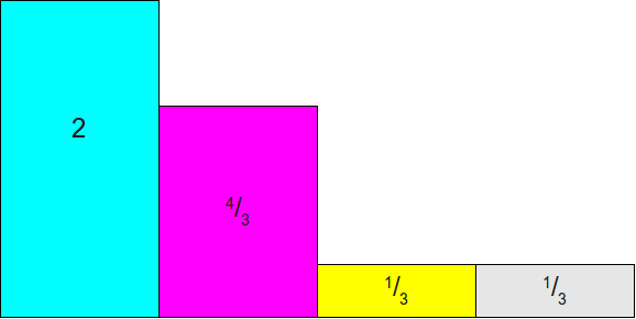
At this point, let's draw a rectangle on top of this image. 1 times4 . It will indicate the target we are shooting at:
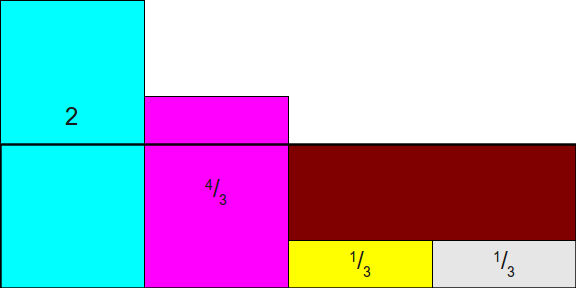
As you can see, this is not entirely correct, because the rectangles for frac12 and frac13 do not fit perfectly into the bounding box. But what if we allow ourselves to cut the rectangles into smaller pieces? That is, what will happen if we cut off part of the space of the rectangle frac12 and move it to the empty space above the space of one of the rectangles 112 ? We will get the following scheme, in which there are still vertical stripes hanging from above, but now there are not so many of them:
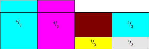
So, we still have extra bands, but not many of them. We could completely eliminate the excess by moving the parts out of the bands.12 and 13into the empty space, but in reality there is a better solution. Let's start by moving12the bars from the first column to the third to fill the remaining space. We will have a small space in the first column, but we will close another space:
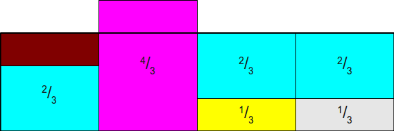
Finally, we will drag the excess from the second column to the first, getting a ready-made rectangle:
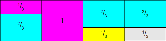
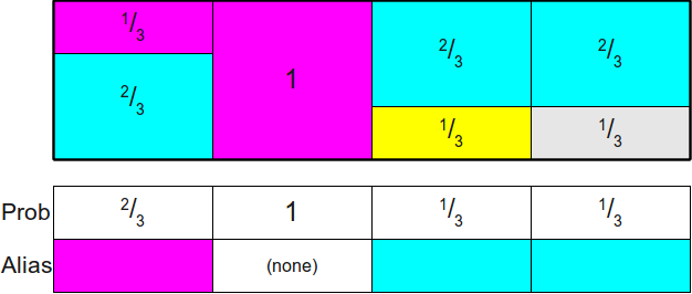
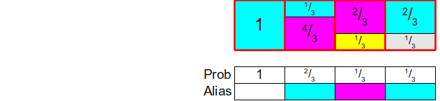
The resulting circuit has remarkable properties. Firstly, the total area of the rectangles. denoting each face of the shulerskoy bone, have not changed compared with the original scheme; we just cut these rectangles into pieces and move them. This means that as long as the areas of the original rectangles are proportionally distributed according to the initial probability distribution, the total area of each face of the bone remains the same. Secondly, notice that there is no free space in this new rectangle, that is, with any dart throw we are guaranteed to get somewhere and get the final answer, and not empty space that requires another throw. This means that a single dart throw will be enough to generate our random value. Last and foremost, notice that each column containsno more than two different rectangles. This means that you can use the previous invention - we throw a bone to choose an asymmetrical coin, and then we throw a coin. The difference this time is in what the throw of the coin means. A dropped eagle means that we choose one face of the bone, and a dropped tails now means that we must choose some other face of the bone (and not throw the bone again).
At a high level, the alias method works as follows. First, we create rectangles that denote each of the different probabilities of the edges of the bone. Next, we cut these rectangles into pieces and redistribute them so that they completely fill the rectangular target so that each column has a constant width and contains rectangles of a maximum of two different sides of the cheat bone. Finally, we simulate the dice rolls, randomly throwing a dart at the target, which can be achieved by combining honest dice and asymmetrical coins.
But how do we know if it is possible to cut the source rectangles at all so that each column contains at most two different probabilities? This does not seem obvious, but it is surprising that this can always be achieved. Moreover, we not only can cut the rectangles into parts so that each column contains no more than two different rectangles, but also make one of the rectangles in each column be the rectangle originally located in this column. You can see that in the rectangle diagram shown above, we always cut out a part of the rectangle and move it to another column and never remove the rectangle of their original column completely. This means that each column in the finished circuit will consist of some kind of rectangle corresponding to the probabilityoriginally assigned to this column, plus (not necessarily) from the second rectangle dragged from some other column. This second rectangle is often calledwith the alias of the column, because the remaining probability of the column is used as the “alias” of some other probability. Due to the use of the term “alias”, this method is called the “alias method”.
Before we get to the proof that you can always distribute probabilities in this way, let's briefly describe the essence of the algorithm. Since each column of the finished scheme always contains some part of the source rectangle from this column (potentially with a zero height!), Then to store (potentially) two different rectangles occupying the column, the implementation of the alias method usually stores two different tables: a probability table Proband alias table Alias . Both of these tables are sized. n .The probability table for each column stores the probability of selecting the source rectangle inside this column, and the identifier of the second rectangle contained in this column (if any) is stored in the alias table. Thus, the generation of a random roll of the bone can be implemented as follows. First, with the help of honest bones, we randomly choose a columni . Next, we throw a random coin with the probability of a falling eagle. Prob[i] . If an eagle has fallen on the coin, then we return that the edge has fallen to the bone. i , otherwise we return that the edge fell on the bone Alias[i] . Here is an example of probability tables and alias for the configuration used above:
Proof of the existence of Alias tables
Now we need to formally prove that the ability to create tables Alias and Probthere is always. To prove that this is always possible, we need to show that it is always possible to do the following:
- Create Rectangles (n⋅pi)×1 for each of the probabilities pi ,
- cut them horizontally into smaller pieces and
- distribute them on n columns
- so that the height of each column is equal 1 ,
- there are no more than two rectangles in one column and
- face rectangle i is located in the column i .
Before turning to the evidence that this is always possible, let's look at an example. Let's say we have four probabilities12 , 13 , 112 , 112 . This is a set of four probabilities ( k=n=4 ), the sum of which is equal to 1=44 .Although we experimentally showed above how to fill in the alias table, now let's consider its creation in more detail and start with a completely empty table, and then begin to fill it. We begin by scaling all these probabilities by a factor of 4, which gives us such probabilities and such an empty table:
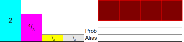
Notice that two of the four rectangles that we need to distribute ( 13 , 13) less than 1. This means that they will not be able to completely fill the column and we need some other probability to fill the rest. Let's take one of the two (let's say yellow) and put it in the appropriate column:
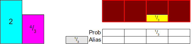
Now we need to somehow cover the difference at the top of the column. To do this, we note that two rectangles that are not yet distributed have a height greater than 1 (namely2 and 43 ).Let's choose one of them arbitrarily; let it be43 . Then we distribute enough of the 43in a column to fill it completely; as a result we will engage23 of 43 as shown below:
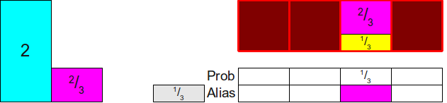
Now let's see what our scheme looks like. We have three rectangles whose total area is equal to3, and three free columns, that is, it seems that these rectangles can be distributed among these three columns. To do this, we use the same trick as before. Note that there is at least one rectangle whose height is less than1 so we will choose one of an arbitrary way (say, a rectangle 23 ) and put it in your column:
Now we need to fill the column to the end, so we take some probability that is not less than 1, and use it to supplement the rest of the column. Here we only have one option (use2 ), so we take 13 of 2 and put it in the upper part of the column:
Now everything has been reduced to two rectangles, the total area of which is two. We repeat this process by finding some rectangle whose height is no more than 1 (here it is13 ), and placing it in this column:
Now we will find some rectangle no less than 1to complete the column. The only option for us is53 :
Now we have only one rectangle left, and its area is 1. Therefore, we can simply complete the creation by placing this rectangle in its own column:
And voila! We have filled the table.
Note that the general pattern underlies the design of this table:
- Find some rectangle whose height is not greater than 1, and place it in its own column, specifying in the table Prob the height of this rectangle.
- Find some rectangle whose height is not less than 1, use it to fill the column, setting the table Alias matching the face of the bone that this rectangle represents.
Is it possible to prove that such a construction is always possible in the general case? That is, that we are not “stuck” by distributing probabilities in this way? Fortunately, there is evidence. This can be explained as follows: we scaled all probabilities so that the average value of the new probabilities is 1 (since initially it was equal to1n , and we multiplied by n ).We know that the minimum of all scaled probabilities should be no more than an average, and that the maximum of all scaled probabilities should be no less than an average, so when we first start from here, we should always have at least one element not more than 1 (namely the smallest of all scaled probabilities) and one element not less than 1 (namely, the largest of scaled probabilities). Therefore, we can pair these elements together. But what happens if we remove them both? When we do this, as a result, we will remove one probability from the total and reduce the total amount of scaled probabilities by one. This means that the new average has not changed, because the average scaled probability is equal. We can repeat this procedure again and again,until we finally pair up all the elements.
We can formalize this reasoning in the following theorem:
Theorem: if availablek unit width rectangles with heights h0 , h1 , ..., hk−1 such that ∑k−1i=0hi=k there is always a way to separate the rectangles and distribute them in k columns, each of which has a height of 1, so that each column will contain no more than two different rectangles, and in i - this column will contain at least one part iof that rectangle.
Proof: by induction. In the base case, ifk=1 , then we have only one rectangle and its height should be equal to 1. Therefore, we can put it in 0th column. Consequently, each column has a height of 1, contains no more than two rectangles, and in0 - this column contains at least one part 0 - .
, - k k+1 1 h0 , h1 , ..., hk , , ∑ki=0hi=k+1 . , hl , , hl≤1 , - hg (, l≠g ), , hg≥1 . , , hl with hl≤1 ; , hi>1 i 0≤i≤k . , k+1=∑ki=0hi>∑ki=01=k+1 , . , - l , , hl≤1 . , hg ( l≠g ), , hg≥1 . , hg<1 , ( ) ∑ki=0hi<k+1 . , hl≤1 and hg≥1 .
. hl l 1−hl at l - hg ( , 0≤1−hl≤1 and hg≥1 ). . k , k , 1 , k+1 . , l , . , , k at k , . , l , , , . .
This is a proof of the possibility of construction, which states that not only can we always build the alias table, but also that the above search algorithm of height is not greater than one and its combination with a rectangle not less than one is always successful. From this we can begin to derive more and more complex algorithms for computing alias tables.
Generating Alias Tables
Using the above, we can get a fairly good algorithm for simulating throws of a cheat bone using the alias method. Initialization consists in a repeated scanning of incoming probabilities to find a value of no more than 1 and a value of no less than 1, followed by combining them into a pair to fill the column:
Algorithm: the naive Alias-method
- Initialization :
- Multiply each probability pi on n .
- Create arrays Alias and Prob each having a size n .
- For j=1 mboxton−1 :
- Find the probability pl satisfying the condition pl le1 .
- Find the probability pg (with l neg ) satisfying the condition pg ge1
- Ask Prob[l]=pl .
- Ask Alias[l]=g .
- Delete pl from the list of initial probabilities.
- Ask pg:=pg−(1−pl) .
- Let be i will be the last remaining probability, which should have a height of 1.
- Ask Prob[i]=1 .
- Generation :
- We generate a roll of honest bones from n - bone; call the face i .
- We throw an asymmetrical coin, dropped by an eagle with probability Prob[i] .
- If an eagle falls on a coin, we return i .
- Otherwise, return Alias[i] .
The step of generating this algorithm is exactly the same as the method described above, and is performed in time Theta(1) . The initialization step requires the multiple iterations described above. First, we need to spend time Theta(n) to scale each probability by a factor n and spend time O(n) on the allocation of two arrays. The inner loop is running Theta(n) times, and with each iteration does the work O(n) by scanning the array, removing one of the elements of the array and updating the probabilities. It gives us time. O(n2) common initialization. If we consider this algorithm in context, then we get the following:
| Algorithm | Initialization time | Generation time | Busy memory | |||
|---|---|---|---|---|---|---|
| The best | Worst | The best | Worst | The best | Worst | |
| Honest bone cheat bone | Theta(n) | O( prodni=0di) | Theta(1) | Theta(n) | O( prodni=0di) | |
| Shuler bone from asymmetrical coins | Theta(n) | Theta(1) | Theta(n) | Theta(n) | ||
| Selection by the roulette wheel | Theta(n) | Theta( logn) | Theta(n) | |||
| The optimal choice of the roulette wheel | O(n2) | Theta(1) | O( logn) | Theta(n) | ||
| Cheat bone of honest bones / asymmetrical coins | Theta(n) | Theta(1) | Theta(n) (expected) | Theta(n) | ||
| Naive Alias Method | O(n2) | Theta(1) | Theta(n) | |||
Compared to other effective simulation methods, this naive alias method has high initialization costs, but then can simulate bone rolls extremely effectively. If we could somehow reduce the cost of initialization (say, up to O(n) ), then this method would definitely be better than all the techniques used here.
One simple way to reduce initialization costs is to use a more appropriate data structure to maintain heights during execution. In the naive version, we use an unsorted array to store all probabilities, that is, it takes time to find the two probabilities we need. O(n) . A more suitable alternative for storing values would be a balanced binary search tree. In this case, we can find the values pg and pl during O( logn) by searching for the maximum and minimum values of the tree. Deletion pl can be done in time O( logn) , and the probability update pg can also be run for O( logn) thanks to its simple removal from the tree, followed by re-insertion. This gives us the following algorithm:
Algorithm: Alias-method
- Initialization :
- Create arrays Alias and Prob each size n .
- Create a balanced binary search tree T .
- We insert n cdotpi at T for every probability i .
- For j=1 mboxton−1 :
- Find and delete the smallest value in T ; let's call him pl .
- Find and delete the highest value in T ; let's call him pg .
- Ask Prob[l]=pl .
- Ask Alias[l]=g .
- Ask pg:=pg−(1−pl) .
- Add pg to T .
- Let be i will be the last remaining probability, which should have a weight of 1.
- Ask Prob[i]=1 .
- Generation :
- We generate a roll of honest bones from n - bone; call the face i .
- We throw an asymmetrical coin, on which an eagle falls on it with probability Prob[i] .
- If an eagle falls on a coin, we return i .
- Otherwise, return Alias[i] .
Now the initialization of our algorithm is much faster. Creature Alias and Prob still takes time O(n) on each table, and adding probabilities to BST T takes time Theta(n logn) . Next we perform Theta(n) iterations to fill the table, each of which takes time O( logn) . This gives us a total initialization time. O(n logn) :
| Algorithm | Initialization time | Generation time | Busy memory | |||
|---|---|---|---|---|---|---|
| The best | Worst | The best | Worst | The best | Worst | |
| Honest bone cheat bone | Theta(n) | O( prodni=0di) | Theta(1) | Theta(n) | O( prodni=0di) | |
| Shuler bone from asymmetrical coins | Theta(n) | Theta(1) | Theta(n) | Theta(n) | ||
| Selection by the roulette wheel | Theta(n) | Theta( logn) | Theta(n) | |||
| The optimal choice of the roulette wheel | O(n2) | Theta(1) | O( logn) | Theta(n) | ||
| Cheat bone of honest bones / asymmetrical coins | Theta(n) | Theta(1) | Theta(n) (expected) | Theta(n) | ||
| Naive Alias Method | O(n2) | Theta(1) | Theta(n) | |||
| Alias method | O(n logn) | Theta(1) | Theta(n) | |||
However, there is an algorithm that works even faster. It is surprisingly simple, and is probably the purest of the alias-method implementation algorithms. This algorithm was first described in the article "A Linear Algorithm For Generating Random Numbers With a Given Distribution" by Michael Vouse, and became the standard algorithm for implementing the alias method.
The basis of the Vouz algorithm is the use of two worklists: one contains elements with a height less than 1, the other contains elements with a height not less than 1. The algorithm constantly connects the first elements of each worklist in pairs. At each iteration, we consume an element from the list of “small” values, and potentially move the rest of the element from the list of “large” values to the list of “small”. This algorithm uses several invariants:
- All items in the small work list are less than 1.
- All items in the “large” worklist are at least 1.
- The sum of the items in the worklist is always equal to the total number of items.
For simplicity, each list stores not the probability itself, but a pointer to a list of initial probabilities, indicating which edge of the cheat bone is being referenced. Having these invariants, we get the following algorithm:
Algorithm: (unstable) Alias-vous method
Warning: this algorithm is subject to numerical inaccuracies. A more numerically stable algorithm is presented below.
- Initialization :
- Create arrays Alias and Prob each size n .
- Create two worklists, Small and Large .
- Multiply each probability by n .
- For each scaled probability pi :
- If a pi<1 add i to Small .
- Otherwise ( pi ge1 ) add i to Large .
- Bye list Small not empty:
- Remove the first item from Small ; call him l .
- Remove the first item from Large ; call him g .
- Ask Prob[l]=pl .
- Ask Alias[l]=g .
- Ask pg:=pg−(1−pl) .
- If a pg<1 add g at Small .
- Otherwise ($ p_g \ ge 1 $) add g at Large .
- Bye list Large not empty:
- Remove the first item from Large ; call him g .
- Ask Prob[g]=1 .
- Generation :
- We generate a roll of honest bones from n - bone; call the face i .
- We throw an asymmetrical coin, on which an eagle falls on it with probability Prob[i] .
- If an eagle falls on a coin, we return i .
- Otherwise, return Alias[i] .
Taking into account the three invariants presented above, the first part of the algorithm (everything except the last cycle) should be fairly clear: we constantly pair in pairs some small element from Small with a large element of Large and then add the rest of the large item to the appropriate worklist. The last loop of the algorithm requires an explanation. After exhausting all the elements in the list Small on the list Large there will be at least one element (since if each element was Small , then the sum of the elements should have been less than the number of remaining elements, which violates the conditions of the last invariant). Because each elment Large not less than 1, and the amount k items in Large must be equal k then every element in Large must be equal to 1, because otherwise the total amount will be too large. Therefore, this last loop sets the probabilities of each large element to 1, so that all columns containing a large element are 1.
In this algorithm, the type of work list is not important. In the original article, Vaugha uses stacks as a worklist because they can be efficiently implemented using arrays, but if we want, we can use a queue. However, for simplicity, we will use the stack.
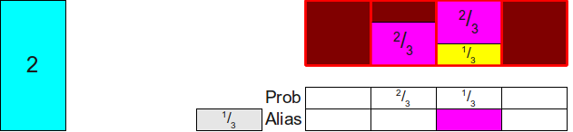
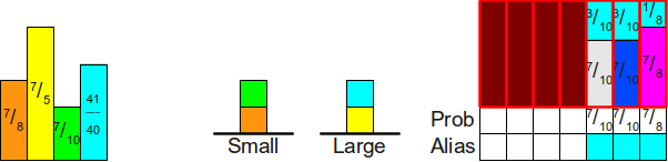
Before proceeding to the analysis of the algorithm, let's analyze its work by example. Consider an example using seven probabilities. frac14 , frac15 , frac18 , frac18 , frac110 , frac110 , frac110 . To emphasize the fact that the algorithm does not sort probabilities and does not require them to be sorted, let's arrange them in arbitrary order. frac18 , frac15 , frac110 , frac14 , frac110 , frac110 , frac18 . The algorithm begins with the addition of these elements in two working stacks:
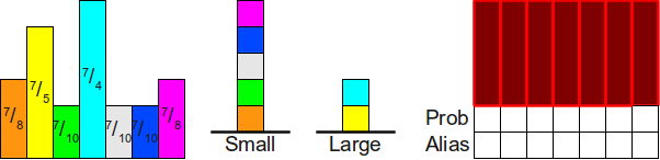
Now we will place the top of the stack Small in its position by moving the lilac rectangle to its final position:
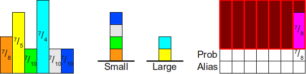
Now we use the top of the stack Large (cyan rectangle) to fill the rest of the column. Insofar as frac74− frac18= frac138 ge1 we leave the turquoise block on top of the stack Large :

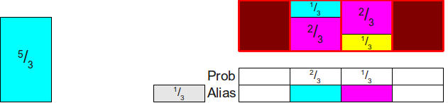
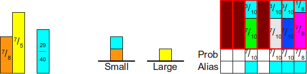
Then we repeat this process. Move the rectangle from the top of the stack Small in its column, and then we add the missing top of the stack Large :
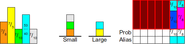
Once again:
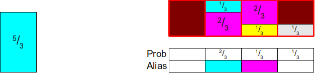
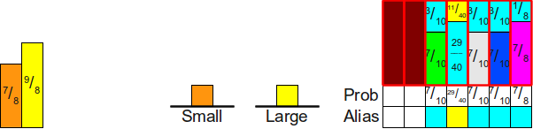
When we repeat this process next time, we find that although we can use the turquoise block to fill in the empty space in the table, but as a result, the height of the turquoise block will become less than one. Therefore, we will need to move the turquoise block to the top of a stack of small values:
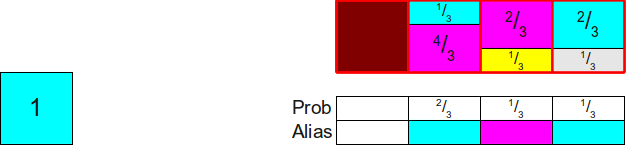
Now when processing the list Small we put a turquoise block in its place, and then use the yellow block to fill the stack:
Then we handle the stack Small To move the orange block to its position, filling the remnants of the yellow block:
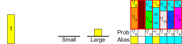
Finally, since the stack Small empty, we put the yellow block in its column and end it.
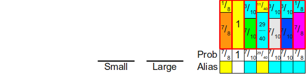
And we have a well-formed alias table for these probabilities.
Practical version of the algorithm of Vouse
Unfortunately, the above algorithm in this form is numerically unstable. It is quite accurate on an idealized machine capable of performing calculations with real numbers of arbitrary precision, but if you try to execute it with the help of IEEE-754 double, then it can be completely erroneous as a result. Here are two sources of inaccuracies that we need to sort out before moving on:
- Calculating whether probability belongs to a worklist Small or to Large may be inaccurate. In particular, a situation may arise in which the scaling of probabilities by a factor n leads to the fact that probabilities equal frac1n , the result is a little less 1 (i.e. get listed Small and not Large ).
- A calculation that subtracts the appropriate probability mass from a higher probability is numerically unstable and can introduce significant rounding errors. This may result in the probability that should be listed Large appears on the list Small .
The combination of these two factors means that as a result, the algorithm can randomly place all probabilities in the list Small instead of a list Large . Therefore, the algorithm may fail, because he expects that when the list Small not empty, then the list Large not empty
Fortunately, this is not so difficult to fix. We will change the internal loop of the algorithm so that it ends when any of the lists is empty, so that we do not accidentally have to search for non-existent elements in the list. Large . Second, when one list is empty, we will assign the remaining probabilities of the elements of the other list to 1 , because from a mathematical point of view, this can only happen when all remaining probabilities are exactly equal 1 . Finally, we will replace the higher probability update calculation with a slightly more stable calculation. Then we get the following:
Algorithm: Alias-Vouse method
- Initialization :
- Create arrays Alias and Prob each size n .
- Create two worklists, Small and Large .
- Multiply each probability by n .
- For each scaled probability pi :
- If a pi<1 add i at Small .
- Otherwise ( pi ge1 ) add i at Large .
- Until Small and Large not empty: ( Large may be devastated first)
- Remove the first item from Small ; call him l .
- Remove the first item from Large ; call him g .
- Ask Prob[l]=pl .
- Ask Alias[l]=g .
- Ask pg:=(pg+pl)−1 . (This is a more numerically stable option. )
- If a pg<1 add g at Small .
- Otherwise ( pg ge1 ) add g at Large .
- Until Large not empty:
- Remove the first item from Large ; call him g .
- Ask Prob[g]=1 .
- Until Small not empty: This is only possible due to numerical instability.
- Remove the first item from Small ; call him l .
- Ask Prob[l]=1 .
- Generation :
- We generate a roll of honest bones from n - bone; call the face i .
- We throw an asymmetrical coin, on which an eagle falls on it with probability Prob[i] .
- If an eagle falls on a coin, we return i .
- Otherwise, return Alias[i] .
The only thing left for us is to analyze the complexity of the algorithm. Creating worklists in general takes time Theta(n) as we add each item to exactly one of the lists. The internal loop runs in time. Theta(1) , because it needs to remove two items from the worklist, update two arrays and add one item back to the list. It can not run anymore. O(n) times, since each iteration reduces the number of elements (total) in the lists by one, eliminating a small probability. Each of the last two cycles can run no more than O(n) because lists Large and Small contains no more O(n) items. This gives us a total lead time. Theta(n) that (as can be seen) is the best result:
| Algorithm | Initialization time | Generation time | Busy memory | |||
|---|---|---|---|---|---|---|
| The best | Worst | The best | Worst | The best | Worst | |
| Honest bone cheat bone | Theta(n) | O( prodni=0di) | Theta(1) | Theta(n) | O( prodni=0di) | |
| Shuler bone from asymmetrical coins | Theta(n) | Theta(1) | Theta(n) | Theta(n) | ||
| Selection by the roulette wheel | Theta(n) | Theta( logn) | Theta(n) | |||
| The optimal choice of the roulette wheel | O(n2) | Theta(1) | O( logn) | Theta(n) | ||
| Cheat bone of honest bones / asymmetrical coins | Theta(n) | Theta(1) | Theta(n) (expected) | Theta(n) | ||
| Naive Alias Method | O(n2) | Theta(1) | Theta(n) | |||
| Alias method | O(n logn) | Theta(1) | Theta(n) | |||
| Alias-vous method | Theta(n) | Theta(1) | Theta(n) | |||
Thoughts in conclusion
Wow! We did a great job! They explored various methods of simulating a cheat bone, starting with the simplest set of techniques and ending with extremely fast and efficient algorithms. Each method demonstrates its own set of techniques, and I consider the final version (the Vouse alias method) to be one of the most interesting and elegant algorithms I have ever encountered.
If you are interested in seeing the code of the alias-method of vous, including a brief description of the difficulties arising in practice due to numerical inaccuracy, then i have an implementation of the alias-method in java , laid out in the archive of interesting code .
I hope the article was useful to you!
Source: https://habr.com/ru/post/419725/
All Articles