Jump Path Search Algorithm
This algorithm is an improved A * pathfinding algorithm . JPS speeds up the search for a path by “jumping over” many places that need to be viewed. Unlike similar algorithms, JPS does not require preprocessing and additional memory costs. This algorithm was introduced in 2011 , and in 2012 received high responses . What is this algorithm and its implementation can be read further in the article.
The algorithm works on the undirected graph of a single value. Each field of the map has <= 8 neighbors that can be passable or not. Each step in the direction (vertically or horizontally) has a value of 1; the diagonal step has a cost of √2. Movement through obstacles is prohibited. The designation refers to one of eight directions of movement (up, down, left, etc.).
“Jump points” allow speeding up the path finding algorithm, considering only “necessary” points. Such points can be described by two simple rules for choosing neighbors in a recursive search: one for rectilinear motion and the other for diagonal. In both cases, it is necessary to prove that excluding the nearest neighbors from a set around a point, there is an optimal path from the ancestor of the current point to each of the neighbors, and this path will not contain the visited point. Consider case 1, which reflects the basic idea:
')
Case 1 : Seperated Neighbor

X is the current point considered. The arrow indicates the direction of travel. And here and there, you can immediately cut off the neighbors, highlighted in gray, because one can get there by the optimal path from p (x), never passing through x.
We will refer to the set of points that remain after clipping the current neighbors of the current point. They are marked in white in the picture. Ideally, we want to consider only true neighbors while watching. However, in some cases, the presence of obstacles may mean that we should also consider a small set of up to K additional points (0 ≤ K ≤ 2). We say that these are points of forced neighbors of the current position.
Case 2 : Forced Neighbor

X is the current point considered. The arrow indicates the direction of travel. Note that when x is next to an obstacle, the selected neighbors cannot be cut off, any alternative optimal path from p (x) at each of these nodes is blocked.
These cases are applied as follows: instead of creating “forced” and “natural” neighbors, we recursively cut off the list of neighbors around each point. Thus, our goal is to eliminate “symmetry,” recursively “jumping over” all points that can be reached through the optimal path that did not pass through the current position. Recursion stops when you hit an obstacle or have found a so-called “jump point successor” (jump point successor). Jumping points are interesting in that they have neighbors that cannot be reached in an alternative way: the optimal way is to go through the current point. Thus, g (y) = g (x) + dist (x; y) is the cost of moving.
To ensure optimality, it is only necessary to decide how to choose neighbors (first linear, then diagonal).
Consider an example:

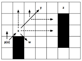
Here you add a point x for consideration, the ancestor of which is p (x); the direction of movement from p (x) to x is a straight-line movement to the right.
(Left picture): Recursively apply the cut-off rule and get y as the successor to the hopping point x. This point is interesting because there is a neighbor z, which can be reached by the optimal path only through y. Intermediate points are not generated and are not considered.
(Right picture): Recursively accept diagonal cutoff rules. Please note that before each next diagonal step, you must recursively walk along straight lines (indicated by a dotted line). Only if both “direct” recursions cannot determine the point of the next jump, then move further along the diagonal. Point w - forced neighbor x, created as usual.
Next, we describe how to cut off the set of points immediately adjacent to some point x. The goal is to find such neighbors, i.e. neighbors (x ), to any n points of which it is impossible to reach the goal optimally. We achieve this by comparing two paths: p, which begins with point p (x), visits x and ends with cn and another way p ', which also begins with p (x), visits x and ends with n, but does not contain x. In addition, each point contained in p or p 'must belong to neighbors (x ).
There are two cases, depending on which transition to x occurs from p (x): a straight move or a diagonal move. It is worth considering that if x is the beginning of p (x), then p (x) is empty and no clipping occurs.
Direct transitions:
Any points are cut off. that satisfy the following statement:
 (one)
(one)
 but
but
Here p (x) = 4 and we cut off all neighbors except n = 5
Diagonal transitions:
Here the differences are that the path that excludes x must be strictly dominant:
 (2)
(2)
 b
b
Here p (x) = 6 and all neighbors are cut off except n = 2, n = 3 and n = 5.
Assuming that neighbors (x) do not contain obstacles, we will refer to the points that remain after the direct or diagonal cutoff (if necessary) as natural neighbors x. They correspond to non-gray dots in a and b figures. When neighbors (x) contain obstacles, it is impossible to cut off all non-natural neighbors. In this case, such a neighbor is considered to be forced (artificial).
Definition 1.
Point is enforced if

 at
at
The example in shows a direct transition, where n = 3 - forced.
 g
g
The example r shows an example of a diagonal movement; here n = 1 is a forced neighbor.
We introduce the definition:
Definition 2.
A point y is a hop point of point x, in the direction d, if y minimizes the value of k such that y = x + kd and one of the following conditions is true:
This figure shows an example of a jump point, which is defined by condition 3. Here we start at point x and end diagonally until we hit point y. From y to z can be reached with k i steps horizontally. Thus, z is the successor of the point for jump x (by condition 2), and this in turn determines y as the successor for jump point x.
Algorithm 1 . Definition of a successor.
Let's set: x - the current point, s - the beginning, g - the goal

Algorithm 1 shows how to find a successor for the current point. First, the set of neighbors immediately adjacent to the current point x is truncated (line 2). Then, instead of adding each neighbor n to the set of successors (successors) for x, we will try to “jump over” to the point that is farther away, but which lies relative to the x direction to n (lines 3-5). For example, if an edge (x; n) is a straight line movement to the right of x, then we look at the jump point directly to the right of x. If there is such a point, then it is added to the set of successors instead of n. If you do not get to the jump point, nothing is added. The process continues until all the neighbors are finished, and then the algorithm returns a list of all the successors for x (line 6).
Algorithm 2 . Jump function.
Let's set: x - a point of the report, d - a direction, s - the beginning, g - the purpose

In order to find individual successors for the jump point, we use algorithm 2. It requires a reporting point x, the direction of motion d, as well as the starting point s and the target point g. The algorithm attempts to establish whether x has a point for jumping among successors by moving in the d direction (line 1) and checks whether the point n satisfies Definition 2. In this case, n is indicated by the jump point and returns (lines 5, 7 and 11). If n is not a jump point, the algorithm repeats recursively and moves again in the d direction, but this time n is a new report point (line 12). Recursion is stopped when an obstacle is encountered and no further actions can be taken (line 3). It should be noted that before each diagonal step, the algorithm must detect jump points in straight directions (lines 9-11). This check corresponds to the third condition of Definition 2 and is important for maintaining the optimality of the algorithm.
Description of the algorithm in the original: harablog.wordpress.com/2011/09/07/jump-point-search
Implementation on js: qiao.github.com/PathFinding.js/visual (select Jump Point Search and arrange the walls)
The code for js: github.com/qiao/PathFinding.js/blob/master/src/finders/JumpPointFinder.js
Benchmark: github.com/Yonaba/Jumper-Benchmark
Detailed visualizer: zerowidth.com/2013/05/05/jump-point-search-explained.html
Terminology and notation
The algorithm works on the undirected graph of a single value. Each field of the map has <= 8 neighbors that can be passable or not. Each step in the direction (vertically or horizontally) has a value of 1; the diagonal step has a cost of √2. Movement through obstacles is prohibited. The designation refers to one of eight directions of movement (up, down, left, etc.).
- Writing y = x + kd means that the point y can be reached in k steps from x in the direction d. When d is a movement diagonally, the movement is divided into two movements in a straight line d 1 and d 2 .
- The path p = (n 0 , n 1 , ..., n k ) is an ordered movement through the points without cycles from the point n 0 to the point n k .
- The notation p \ x means that the point x does not occur on the path p.
- The notation len (p) means the length or cost of the path p.
- The notation dist (x, y) means the length or cost of the path between points x and y.
Jump points
“Jump points” allow speeding up the path finding algorithm, considering only “necessary” points. Such points can be described by two simple rules for choosing neighbors in a recursive search: one for rectilinear motion and the other for diagonal. In both cases, it is necessary to prove that excluding the nearest neighbors from a set around a point, there is an optimal path from the ancestor of the current point to each of the neighbors, and this path will not contain the visited point. Consider case 1, which reflects the basic idea:
')
Case 1 : Seperated Neighbor
X is the current point considered. The arrow indicates the direction of travel. And here and there, you can immediately cut off the neighbors, highlighted in gray, because one can get there by the optimal path from p (x), never passing through x.
We will refer to the set of points that remain after clipping the current neighbors of the current point. They are marked in white in the picture. Ideally, we want to consider only true neighbors while watching. However, in some cases, the presence of obstacles may mean that we should also consider a small set of up to K additional points (0 ≤ K ≤ 2). We say that these are points of forced neighbors of the current position.
Case 2 : Forced Neighbor
X is the current point considered. The arrow indicates the direction of travel. Note that when x is next to an obstacle, the selected neighbors cannot be cut off, any alternative optimal path from p (x) at each of these nodes is blocked.
These cases are applied as follows: instead of creating “forced” and “natural” neighbors, we recursively cut off the list of neighbors around each point. Thus, our goal is to eliminate “symmetry,” recursively “jumping over” all points that can be reached through the optimal path that did not pass through the current position. Recursion stops when you hit an obstacle or have found a so-called “jump point successor” (jump point successor). Jumping points are interesting in that they have neighbors that cannot be reached in an alternative way: the optimal way is to go through the current point. Thus, g (y) = g (x) + dist (x; y) is the cost of moving.
To ensure optimality, it is only necessary to decide how to choose neighbors (first linear, then diagonal).
Consider an example:
Here you add a point x for consideration, the ancestor of which is p (x); the direction of movement from p (x) to x is a straight-line movement to the right.
(Left picture): Recursively apply the cut-off rule and get y as the successor to the hopping point x. This point is interesting because there is a neighbor z, which can be reached by the optimal path only through y. Intermediate points are not generated and are not considered.
(Right picture): Recursively accept diagonal cutoff rules. Please note that before each next diagonal step, you must recursively walk along straight lines (indicated by a dotted line). Only if both “direct” recursions cannot determine the point of the next jump, then move further along the diagonal. Point w - forced neighbor x, created as usual.
Neighbor cut rules
Next, we describe how to cut off the set of points immediately adjacent to some point x. The goal is to find such neighbors, i.e. neighbors (x ), to any n points of which it is impossible to reach the goal optimally. We achieve this by comparing two paths: p, which begins with point p (x), visits x and ends with cn and another way p ', which also begins with p (x), visits x and ends with n, but does not contain x. In addition, each point contained in p or p 'must belong to neighbors (x ).
There are two cases, depending on which transition to x occurs from p (x): a straight move or a diagonal move. It is worth considering that if x is the beginning of p (x), then p (x) is empty and no clipping occurs.
Direct transitions:
Any points are cut off.
that satisfy the following statement: (one) butHere p (x) = 4 and we cut off all neighbors except n = 5
Diagonal transitions:
Here the differences are that the path that excludes x must be strictly dominant:
(2) bHere p (x) = 6 and all neighbors are cut off except n = 2, n = 3 and n = 5.
Assuming that neighbors (x) do not contain obstacles, we will refer to the points that remain after the direct or diagonal cutoff (if necessary) as natural neighbors x. They correspond to non-gray dots in a and b figures. When neighbors (x) contain obstacles, it is impossible to cut off all non-natural neighbors. In this case, such a neighbor is considered to be forced (artificial).
Definition 1.
Point
is enforced if atThe example in shows a direct transition, where n = 3 - forced.
gThe example r shows an example of a diagonal movement; here n = 1 is a forced neighbor.
Algorithm Description
We introduce the definition:
Definition 2.
A point y is a hop point of point x, in the direction d, if y minimizes the value of k such that y = x + kd and one of the following conditions is true:
- The point y is the destination.
- Point y has at least one neighbor that is constrained by definition 1.
- d - movement on the diagonal and there is a point z = y + k i d i , which lies in k i steps in the direction d i ∈ {d1, d2}, such that z is a jump point from y under condition 1 or 2.
This figure shows an example of a jump point, which is defined by condition 3. Here we start at point x and end diagonally until we hit point y. From y to z can be reached with k i steps horizontally. Thus, z is the successor of the point for jump x (by condition 2), and this in turn determines y as the successor for jump point x.
Algorithm 1 . Definition of a successor.
Let's set: x - the current point, s - the beginning, g - the goal
Algorithm 1 shows how to find a successor for the current point. First, the set of neighbors immediately adjacent to the current point x is truncated (line 2). Then, instead of adding each neighbor n to the set of successors (successors) for x, we will try to “jump over” to the point that is farther away, but which lies relative to the x direction to n (lines 3-5). For example, if an edge (x; n) is a straight line movement to the right of x, then we look at the jump point directly to the right of x. If there is such a point, then it is added to the set of successors instead of n. If you do not get to the jump point, nothing is added. The process continues until all the neighbors are finished, and then the algorithm returns a list of all the successors for x (line 6).
Algorithm 2 . Jump function.
Let's set: x - a point of the report, d - a direction, s - the beginning, g - the purpose
In order to find individual successors for the jump point, we use algorithm 2. It requires a reporting point x, the direction of motion d, as well as the starting point s and the target point g. The algorithm attempts to establish whether x has a point for jumping among successors by moving in the d direction (line 1) and checks whether the point n satisfies Definition 2. In this case, n is indicated by the jump point and returns (lines 5, 7 and 11). If n is not a jump point, the algorithm repeats recursively and moves again in the d direction, but this time n is a new report point (line 12). Recursion is stopped when an obstacle is encountered and no further actions can be taken (line 3). It should be noted that before each diagonal step, the algorithm must detect jump points in straight directions (lines 9-11). This check corresponds to the third condition of Definition 2 and is important for maintaining the optimality of the algorithm.
Links
Description of the algorithm in the original: harablog.wordpress.com/2011/09/07/jump-point-search
Implementation on js: qiao.github.com/PathFinding.js/visual (select Jump Point Search and arrange the walls)
The code for js: github.com/qiao/PathFinding.js/blob/master/src/finders/JumpPointFinder.js
Benchmark: github.com/Yonaba/Jumper-Benchmark
Detailed visualizer: zerowidth.com/2013/05/05/jump-point-search-explained.html
Source: https://habr.com/ru/post/162915/
All Articles