L-systems. Tree modeling

The post is a free translation of the second chapter of the book “Algorithmic Beauty of Plants” by Przemyslav Prushchinkevich and Aristide Lindenmayer (The Algorithmic Beauty of Plants, Aristid Lindenmayer, Przemyslaw Prusinkiewicz), and is a continuation of the wonderful article “ L-Systems - the mathematical beauty of plants ” valyard (thanks to him for inspiration :)

The first models.

Computer modeling of tree branching processes has a relatively long history. The first model proposed by Yulem was based on the concept of cellular automata developed by von Neumann. The branching process was carried out by iterations, and began with one colored cell on a triangular grid, then those that touched one and only one vertex of the cells that were painted in the previous iteration were painted.

Further, this idea was developed. Meinhardt replaced the triangular square grid, and used the resulting cellular space to test the biological hypotheses of the formation of network structures. In addition to the pure branching process, his model took into account the effects of repeated connections or anastomosis that could occur between leaves or, for example, veins. Green rewrote the cellular automaton for three dimensions and modeled growth processes that took into account the environment. For example, Figure 2.1 shows the growth of a vine over a house. Cohen's models took into account the concept of "field density" in the growth rules, which turned out to be better than, for example, working with discrete cells.
')

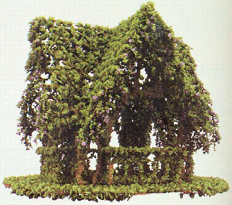
Figure 2.1. Harmonious Green architecture.

A common feature of these approaches is the emphasis on the interaction, both between different elements of the structure and the structure with the environment. And although this interaction obviously affects the growth of real plants, its modeling is a very difficult task. Therefore, simple models are now more common, ignoring even such fundamental things as collision between branches.

Honda model.

Honda proposed the first model in the category of simple, and made the following assumptions:

• tree segments are straight, their cross-sectional area is not considered;
• during the iteration, the parent segment produces two children;
• the length of two child segments is shorter than the maternal and time;
• the parent segment and its two subsidiaries are in the same branch plane . Child segments out of the parent at branch angles and ;
• in connection with the action of gravitational force, the branch plane is “closest to the horizontal plane”, in other words, the line perpendicular to the parent segment and lying in the plane of the branch is horizontal. An exception is made for branches attached to the main trunk. In this case, a constant angle of divergence is used. .

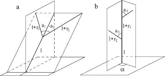
Figure 2.2. Tree geometry according to Honda.

Varying numerical parameters, Honda received a wide variety of tree-like forms. With some improvements, his models were applied to the study of branching processes of real trees. Subsequently, different rules for branch angles were proposed in order to also cover tree structures in which the planes of further ramifications are perpendicular to each other. Honda's results served as the basis for the models proposed by Eono and Kyuniai. They proposed several improvements, the most important of which was the rotation of the segments in certain directions, corresponding to the aspiration of the branches to the sun, taking into account wind and gravity. A similar concept was proposed by Cohen, and Refay and Armstrong developed a more physically accurate branch bending method.

In the models of Honda, Eono and Kuniyay, straight lines of constant or variable width were used to construct the "wood skeleton". Significant improvements in the photorealism of the synthesized models reached Blumenfel and Oppenheimer, which presented curving branches, carefully modeled the surfaces around the branch nodes, and applied textures to the bark and leaves (Figure 2.3)


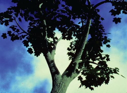
Figure 2.3. Blumenfel, Acer graphics.

In Honda’s work, the branch structure was constructed according to deterministic algorithms. In contrast, in the group of models proposed by Reeves and Blau, de Refay, Remfrey, Neill and Steves, stochastic laws were used. Although these models are built differently, they share a common paradigm for describing the structure of trees, in particular, the calculation of the possibilities of forming branches. Reeves and Blau sought not to delve into the biological details of the simulated structures (Figure 2.4). In contrast, de Refay used a stochastic approach to create realistic plants and simulated kidney activity at discrete points in time. Having received the timer signal, the kidney could either:

• nothing to do;
• become a flower;
• become a segment of the stem, ending with a new apex and one or more side branches of the stem;
• die or disappear.

These events occurred according to the stochastic laws described separately for each plant species. Geometrical parameters, such as the length and diameter of the stem segment, the angles of branching, were also calculated according to stochastic algorithms.


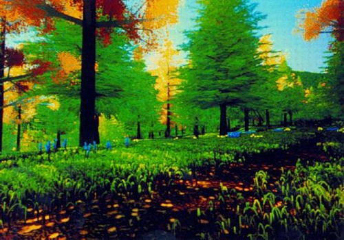
Figure 2.4. Picture of the Forest, Reeves, © 1984 Pixar.


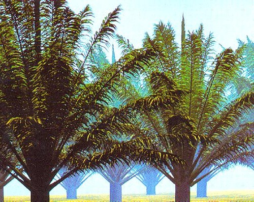
Figure 2.5. Oil palm shelter, CIRAD Modelisation Laboratory.

Using the basic types of development laws in this method, Helle, Oldemen, and Tomlinson established 23 different types of tree architecture. Detailed models of selected plant types are developed and described in the literature. A simple tree model is shown in Figure 2.5. The approach of Remfrey was similar to the approach of de Refay, but the first used longer time intervals. It turned out that in order to achieve reliable results, stochastic models should describe the behavior of lateral shoots, which is possible during the year.

The use of L-systems for generating trees was first considered by Eono and Kyunai. For a start, based on the formal definition of L, they proved its unsuitability for modeling higher plants. But the proof did not apply to parametric L-systems with snail interpretation of strings. For example, the L-systems in Figure 2.6 performs those Honda models in which one of the branch angles is zero, the pliable monopodial structure and the clearly defined main and side axes.


Figure 2.6. Tree models with monopodial branching of Honda, obtained on L-systems.

n = 10
#define r1 0.9 /* */
#define r2 0.6 /* */
#define a0 45 /* */
#define a2 45 /* */
#define d 137.5 /* */
#define wr 0.707 /* */
ω : A(1,10)
p1: A(l,w) : *→ !(w)F(l)[&(a0)B(l*r2,w*wr)]/(d)A(l*r1,w*wr)
p2: B(l,w) : *→ !(w)F(l)[-(a2)$C(l*r2,w*wr)]C(l*r1,w*wr)
p3: C(l,w) : *→ !(w)F(l)[+(a2)$B(l*r2,w*wr)]B(l*r1,w*wr)

* This source code was highlighted with Source Code Highlighter .

Table 2.1. The constants for monopodial tree structures in Figure 2.6.

Note per. - here it is interesting that the thickness of the segments between the nodes of the tree should be constant, and the picture shows that the thickness of the trunk begins to decrease even before the first branching, which contradicts the previous and subsequent arguments. Not seen on other pictures :)

According to the expression , with each iteration from the top of the main axis stem segment leaves and side top . Constants and indicate a decrease in length for the straight and lateral segments, and - branch angles and - angle of divergence. Module sets the line width so the expression reduces the width of the child segments from the parent to time. This constant satisfies the postulate of Leonardo da Vinci, according to which the total thickness of all branches folded together in any cross-section of a tree with a horizontal plane is equal to the thickness of the trunk under them. In case from the parent branch diameter , there are two children of equal diameter This postulate gives the equation hence the value equally .

Note per. - under the thickness of the branches and the thickness of the trunk, you should probably understand their cross-sectional area, then it becomes clear where the squares appeared in the last equations.

Expressions and describe the further development of the side branches. At each iteration, a straight vertex ( or ) releases the next-sided vertex at an angle or in relation to the maternal axis. Both expressions are used to create side vertices alternately left and right. Symbol rotates a turtle around its own axis, with the vector indicating the direction of "left" turtles held horizontally. Consequently, the branch plane is “closest to the horizontal plane,” as is required in the Honda model. Writing in vector form, changes the orientation of the bug in space according to:




where are the vectors , and - the main, left and top vectors attached to the bug, - vector directed in the opposite direction from the direction of gravity. Figure 2.6 shows trees that are modeled with the constants listed in Table 2.1 and coincide with the Honda tree models.

Simpodial branching.

Other L-systems, shown in Figure 2.7, cover the sympodial structures in which both child segments form a nonzero angle with the parent. In this case, the activity of the main peak is reduced due to the formation of the trunk. and pairs of side vertices (expression ). Further branching is done by . The simple structures in Figure 2.7 were obtained using the constants listed in Table 2.2, and correspond to the models presented by Eono and Kyunai.



Figure 2.7. Models of trees with sympodial branching Eono and Kyuniai, obtained on L-systems.

n = 10
#define r1 0.9 /* 1 */
#define r2 0.7 /* 2 */
#define a1 10 /* 1 */
#define a2 60 /* 2 */
#define wr 0.707 /* */
ω : A(1,10)
p1 : A(l,w) : *→ !(w)F(l)[&(a1)B(l*r1,w*wr)]
/(180)[&(a2)B(l*r2,w*wr)]
p2 : B(l,w) : *→ !(w)F(l)[+(a1)$B(l*r1,w*wr)]
[-(a2)$B(l*r2,w*wr)]

* This source code was highlighted with Source Code Highlighter .

Table 2.2 Constants for trees with sympodial branching in Figure 2.7.


The previous models have a somewhat artificial character, because the final length of each segment is set even when it is created, and does not change in subsequent iterations. But it is possible to simulate the growth process itself, that is, to increase the length and width of the parent segments with the growth of the subsidiary. An example of an L-system constructed according to this paradigm is given in Figure 2.8.

Ternary branching.

The overall structure of the tree is defined by the expression . At each iteration, the vertex produces 3 new branches ending in their own vertices. Parameter and constant determine the ratio of the width of the parent branch to the width of the child branch . According to da Vinci's postulate , in this way, . Expressions and describe a gradual change in the length of the branches and an increase in their diameter.



Figure 2.8. Models of trees with ternary branching.

#define d1 94.74 /* 1 */
#define d2 132.63 /* 2 */
#define a 18.95 /* */
#define lr 1.109 /* */
#define vr 1.732 /* */

ω : !(1)F(200)/(45)A
p1 : A : *→ !(vr)F(50)[&(a)F(50)A]/(d1)
[&(a)F(50)A]/(d2)[&(a)F(50)A]
p2 : F(l) : *→ F(l*lr)
p3 : !(w) : *→ !(w*vr)

* This source code was highlighted with Source Code Highlighter .

Table 2.3. Constants for tree models in Figure 2.8.


Tropism is the reaction of an organism, for example a plant, to an external influence by growth in the direction determined by this influence. In particular, the desire of plants to light manifests itself in the form of twisting branches. This is modeled by a slight turn of the turtle after drawing each segment in the direction determined by the vector of tropism. (Figure 2.9). The angle of rotation a is calculated using the formula = | where - A parameter characterizing the sensitivity, susceptibility of the axis to rotation. This formula has a physical explanation: if interpreted as a force applied to the end of the vector and can rotate around its starting point, then the torque is equal to . Parameters related to the generation of tree models in Figure 2.8 are listed in Table 2.3. A realistic render of a tree in Figure 2.8d is shown in Figure 2.10.


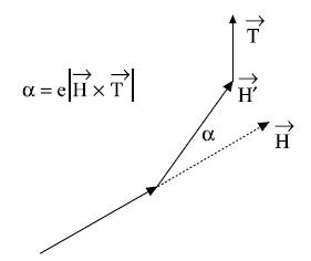
Figure 2.9. Correction segment thanks to tropism .


Figure 2.10. Charming Lake Musgrave et al.


Figure 2.11. Surreal elevator.

Conclusion

The examples above show that models of Honda trees, like the models of his followers Eono and Kyuniai, can be obtained using L-systems. Shebell also showed that L-systems can play an important role as a tool for biologically-correct tree modeling and the synthesis of photo-realistic images. However, while the models obtained are of a general nature, and the structures of specific trees are still in development. L-systems are also widely used in the realistic modeling of herbal plants discussed in the next chapter.

---

PS If the “photo-realistic” images from the 1990 book do not deliver, then perhaps more modern renders from another article ( pdf ) on algorithmicbotany.org will seem interesting:


PPS The translation does not provide an infinite number of references to the literature, which is in the original book. The numbering of tables and pictures is left original. The original of the book is here: algorithmicbotany.org/papers/#abop . If the site is lying, the book in pdf can be downloaded here: all , only the second chapter . If in the text there are spelling / technical errors, please immediately inform the PM))