Effective segmentation of images on graphs

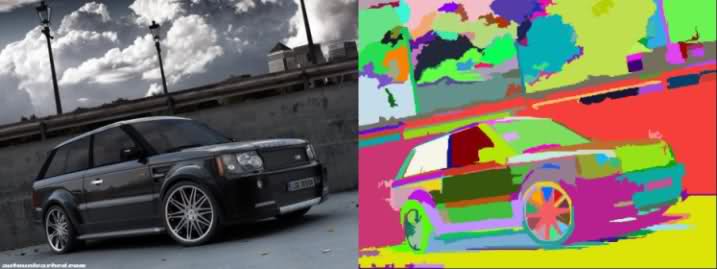
Image segmentation and object detection ( edge detection ) play an important role in Computer Vision systems and are used for scene recognition and object selection (detection) tasks. By and large, this is the same tool as, for example, sorting, designed to solve higher-level problems. And therefore, an understanding of the device of this class of algorithms will not be superfluous when building such systems, taking into account the requirements (in terms of quality / performance) and the specifics of the tasks.

This article briefly describes the “Efficient Graph-Based Image Segmentation” algorithm by Pedro F. Felzenszwalb ( MIT ) and Daniel P. Huttenlocher ( Cornell University ), published in 2004. Yes, the algorithm is relatively old, but despite this, it still remains very popular, showing good results in terms of performance.

Under the cut - a large mixture of pictures and text, not demanding to the current level of knowledge of the subject. Curiosity is welcome .
')


First, the algorithm on the graphs, at first glance, having little in common with image processing, will be described. However, a little later it will be given its interpretation in relation to image segmentation.

Kruskal Algorithm

The Kraskal algorithm ( wiki ) builds a framework - the minimum spanning tree of a given graph. Further the English abbreviation MST (minimum spanning tree) will be used.

Task: there are several settlements on the map (there are several contacts on the board), it is necessary to connect all of them with each other in such a way that the total length of roads (wires) is minimal.


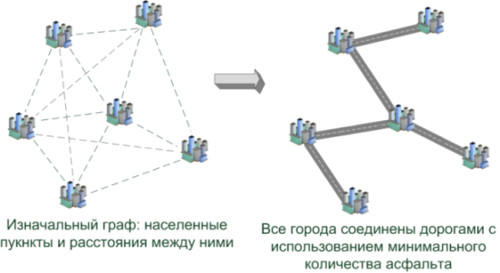
* Yes, a task in such a formulation is usually called the “Steiner task” ( article ), having solved which, cities can be connected even cheaper. But we, ultimately, do not lay the asphalt ... =)

For the solution will need:

• Counts : Briefly about what it is and how they are represented in the code has already been described in Habré ( article )
• Kraskal's algorithm ( wiki ): the main “engine” for solving the problem in such a formulation. He is very well described in Cormen’s, Leiserson’s bible “Algorithms: Construction and Analysis” ( book )
• Disjoint-set data structure ( wiki ): an additional structure necessary for the efficient implementation of the above algorithm. How it is arranged, described in the same bible, but only slightly under a different name ( if memory serves: Union Find-Set, something like that )

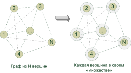
In the current formulation of the problem, the vertices of the graph (v _i ) are cities, and the edges e (v _i , v _j ) are roads between cities. We know the distances between pairs of cities (v _i , v _j ) - this is the weight of the edges w (e (vi, vj)) . Need to find MST, i.e. is a tree in the graph (without cycles: why build extra roads) so that the sum of the edges is minimal and at the same time all the vertices are reachable.

Initially, each vertex (city) itself is the only proud representative of the corresponding set G ₁ , G ₂ , ... G _N (by the number of vertices). Let him think so far that it was she who formed the MST. In the course of the algorithm, we effectively and diplomatically combine all these separate sets into a single G so that the participating vertices form the MST. For this:

• Sort all the edges in the graph in ascending order of length (road)
• Running along the edges in ascending order of lengths, we look at the ends of the edge e = (a, b) :
  • If the vertices ( a and b ) belong to the same set : So, they already participate in some educated subset of the micro-MST, within their subgraph the sum of the edges is already minimal. This edge is skipped - we don’t need it. otherwise it forms a cycle in the tree, and we will use up asphalt for nothing
  • If the vertices ( a and b ) belong to different subsets of the micro-MST: we have found an edge (road) of minimal length, combining (merging) both subsets into one. All the edges of smaller length have already been considered and cheaper than this edge, it will not be possible to combine. Such an edge is entered in the list of edges used in constructing the MST tree, and the sets are combined into one
  • Continue the merge cycle to obtain a single set equal to the desired MST, which will contain all the vertices of the graph
• We get one single set of vertices (MST) and a list of edges used to join it, which is a tree of minimum total length, which unites all vertices.

Disjoint-set data structure

To implement the concept of “set” in the Kraskal algorithm, the Disjoint-set data structure is used . Work with it is optimized to perform two basic operations:

• Find out for some vertex which set it belongs to at the moment
• Quickly merge these sets into one

To get closer to the topic of image segmentation, the description will continue in terms of image pixels and their colors. Suppose we segment a parrot against the backdrop of some Japanese blue sea. At first, each pixel (vertex of the graph) will be by itself - in its own segment (set), but during the algorithm, the pixels (vertices) of the "similar" color (one object) are gradually merged into one segment.

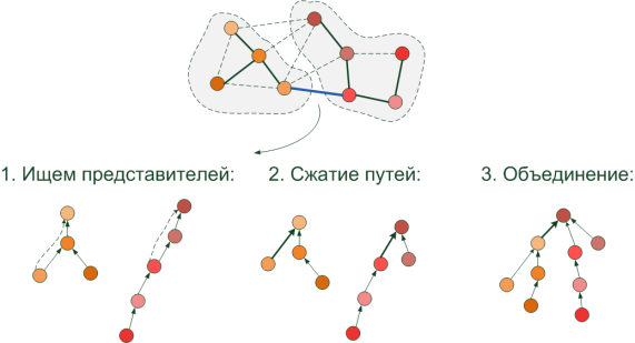
For example, at a certain step of the algorithm, there is an edge connecting two neighboring pixels: at one end of the edge, the pixel is “orange”, and at the other “red”. The edge length is defined as the “color difference” between pixels. All the edges of smaller length (with a similar color) are already merged: the orange and red parrot segment is probably already selected. Following the algorithm, we need to find out if the current “orange” and “red” pixel are in one segment? If in different, and we believe that the segments are similar in color, then we combine them into one and continue to build ... In general, the same algorithm of Krasalka, only with pixels.

The structure used for these operations is very similar to the tree (although it is implemented by an array of indices). It contains an ancestor for each pixel, i.e. pointer (index) to some pixel of similar color located in the same segment. Basic operations:

• Search for a segment of a certain pixel 'x' : go through the ancestors to the very top. The topmost pixel is the root of the tree, the “representative” of this segment at the current moment.
• Merge segments . If the pixels have different “representatives”, then they belong to different segments, otherwise the root would be the same. To combine the “representative” of a segment of lesser height (from the farthest pixel to the root), we refer (specify from it) to a longer “representative” in order not to increase the height of the tree. Now we have a combined segment with a common representative.
• In order not to run the next time far from the pixel to the root, after the “representative” is successfully detected, we establish a direct link from the pixel — right to it. This shortens the path of the following searches, and is called " path compression ".

Great, now we can effectively search for segments by pixels and merge them, as well as build MST using the Kraskal algorithm. It is time to learn how the decision is made to merge or split the two areas.

Divide and rule

The segmentation algorithm must clearly define where one segment ends and another begins. As a rule, the borders are characteristic drops of brightness and / or hues of color found on the object-background, plane-shadow, parrot-sea, sign on the fence ... And if the "drop" is greater than a certain "threshold", then This should follow that these are different segments. But there is a small problem: drops can vary greatly for different objects, and it is difficult to “separate” the segments with a uniquely defined (const) threshold value (threshold). For the surface of the table on the background of the wall: the differences of neighboring pixels along the surface of the table (wall) will be relatively small, but on the table-wall border there will be a jump, which will separate the segments. It is clear. And if we have a parrot on the background of the sea? He himself is very "motley", inside him there are large differences in intensity (green-red-yellow -...), in order to "separate" him from the sea, we need another "threshold" (threshold). And we gradually come to the conclusion that the threshold, which decides that the neighboring segments "cannot be together," should be based not only on local indicators: the intensity difference along one edge (connecting neighboring pixels), but also on how much these segments on their own smooth (in terms of color) or "variegated".

Gray pictures

Before proceeding to the processing of full-color images, consider a simplified version, when the image is represented by grayscale, i.e. Each cell of the image matrix stores a number in the interval [0 ... 1] , which represents the pixel brightness.

Efficient Graph-Based Image Segmentation

Each pixel of the image is represented by a vertex in the graph. And the weight (length) of the edge connecting adjacent vertices is expressed by the formula: w (v _i , v _j ) = | I (p _i ) -I (p _j ) | where I (p _i ) is the intensity (brightness) of the pixel p _i

During the execution of the Kraskal algorithm, at the intermediate stage we will have several separate segments (subsets of pixels) with the minimum total weight of the edges inside: the segments will be joined by edges of the minimum length, i.e. with minimal "intensity differences" between adjacent pixels. Therefore, adjacent pixels inside one segment will be similar in color. But only up to a certain value of the maximum edge (differential intensity) ...

And so ... we took the minimum edge in the current step. For two pixels, which are adjacent vertices of this edge, can we determine from one (already constructed) segment?

• Yes , from one segment: just continue the execution of the algorithm.
• No It is necessary to determine whether the segments represent parts of the same object in the image and should they be combined, or do their intensities “substantially” differ?

To determine the differences between the segments, with each already constructed segment we associate a certain quantity — the maximum intensity difference inside it, i.e. longest edge in MST inside a segment:

Separately, it’s not necessary to look for it - it’s enough just to keep the edge length added when combining the components of the “sub-segments”. Indeed, at the time of combining, the length of the added edge was greater than in the already constructed MST of each “sub-segment”, since edges are processed in ascending order.

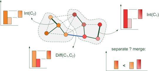
We obtain an approximate decision rule for segments C ₁ , C ₂ :

	Sign: whether these segments should be delimited
	The current edge of the minimum length connecting two separate segments
	Smaller (of the larger) intensity differences within one of the considered segments

It turns out that , in order for the segments to “merge,” the intensity difference at their border must be less than the maximum differential within each of the segments being merged:

I am looking for you

How to build a graph in the image? Which pixels are adjacent? On the surface are two main approaches:

• 4-connected : we connect each pixel with the adjacent top / bottom / left / right. Such a construction is attractive because the number of edges in the graph is minimal.
• 8-connected : in addition to the previous version, we connect each pixel with the neighboring ones located diagonally. Thus, there are more edges in the graph, the algorithm runs slightly slower. But the resulting segmentation should be of higher quality - after all, more connections between the pixels are taken into account.

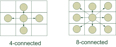
The algorithm should give better results on the 8-connected constructed graph, however 4-connected gives very acceptable results and at the same time it runs much faster. And as a “distance” for processing color images we can take just such a simple color difference of pixels, as realized by the authors of the algorithm:

However, this distance formulation has a flaw. If we consider the “intensity drop” between locally adjacent pixels, then the sky in the next picture will be divided into 2 separate segments with a wire passing across, or we will get even worse result if we process the lawn against the background of the grid:


Each piece of the lawn will be marked as a separate segment, but this is one object!

Therefore, in the alternative, the authors propose to consider not only the nearby pixels, but pushing away from the local properties of the image (pixels located in close proximity), try to “jump over the wire” (see the picture) and reach for the continuation of a segment located at some distance. To do this, they suggest choosing the Euclidean distance as the edge length, depending on both the position of the pixels (x, y) and their color (r, g, b) :

Now the pixels will be considered “neighbors” if they are located close to each other, or have a similar shade, although they may physically be at some distance. For the construction of the graph, the authors propose to connect each pixel with 10 (20, 30) "closest" ones. This gives better segmentation, but requires more computational resources.

Stick together, team!

Returning to the very beginning. A long time ago, when all the pixels were scattered — there could be a significant difference in intensity between the neighboring ones, which did not allow them to merge. It is unlikely that they provided us with a microscopic photograph, where each pixel should be isolated - most likely, they are part of some larger object (parrot). So that they succumb to the "merge" (merge) to a greater extent than the already built large segments, for which the correctness of the splitting is more important, add a value in the final rule depending on the size of the constructed segment: where | C | - power of the considered segment (the number of pixels in it at the current moment), and k is already a segmentation parameter set manually. With a similar amendment in the final rule, the formula will be used:


The “amendment” is gradually leveled with the growth of the segment (increase | C | ) ...

In fact, instead of this task T, you can choose another function that takes into account the specificity of the processed images: the shape of the segments, the position in the photo, certain color shades ...

Gaussian blur

Returning to the very "colorful" pictures:


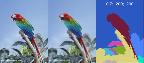
It is clear that when determining the distance between pixels in such a definition as “intensity difference”, the pixels of a “motley”, even if a single object, will not be very flexible to merge into one object. To make them more “compliant” to combine and remove noise / artifacts, a Gaussian blur filtering (http://habrahabr.ru/blogs/webdev/43895/) is usually applied to the image with a certain radius (standard deviation) of sigma . This causes the "interpenetration" of the color components of the pixels, and they are more willing to contact.

Total

There are many methods for segmentation: various approaches are very well described in the article “Image segmentation methods: automatic segmentation”. And by and large, the segmentation must be either qualitative or productive, and if you are lucky, all at once. The method described above is exactly the productive version.

In this way of segmentation, the most laborious process is the sorting of all edges performed in O (e log ⁡e) , where e is the number of edges in the graph. Thus, for an image of NxM pixel edges will be: | e | = 4 * N * M

The source code of the algorithm is available at this link .

But what about OpenCV?

In all of your favorite OpenCV library ( wiki ) there is a method " cvPyrSegmentation ", i.e. pyramidal image segmentation method. It is arranged a little differently. His description would take another article, so - the picture. Segments are built in layers (level), combining pixels of similar color into one (located in a layer above), and then sequentially processing the layers located at the next level (level) above “against the stop”:


In 2006, a comparison of several pyramidal algorithms was carried out in the Univesity of Malaga (Spain) and the results are presented in the following article :


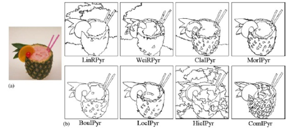
The authors came to the conclusion that of the 8 methods that deserve attention are 3, thanks to which sufficiently high-quality results of image splitting into objects are obtained. However, it is worth noting that the execution time of the pyramidal algorithms varies from 0.5 sec. up to 4.5 seconds (256x256 pixels on a Pentium 766 MHz), while the considered " Efficient Graph-Based Image Segmentation " is performed according to the words of the authors "in fraction of a second". We have 1024x768 photos worked for 0.5 seconds (U9400 2 x 1.4GHz) inside the "matryoshka": VMWare - Matlab - mex (C ++). In general, pyramidal - the quality described in the article columns - speed. Both have the right to life. =)


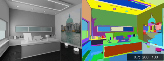
To the most assiduous readers, let us reveal the secret of the “magic bubbles”: what kind of numbers are depicted in the pictures? These are just the parameters of the " segmentation (sigma, k, min) " method, with 2 of which you are already familiar with, and the 3rd " min " is the enforced minimum segment size so that there are no "small" ones.


Good luck!

PS Please do not kick much, this is my ninth post on Habré.