Python cluster analysis
The wonderful book “We Program Collective Mind” inspired me to write this post based on her motives on cluster analysis.
There was a desire in one post to consider cluster analysis, its beautiful implementation in Python, and, especially, the visual representation of clusters - dendrograms .
The code of the example is based on the code of the examples from the book.
')
The main idea of cluster analysis is the selection among a multitude of data groups within which the elements are to some extent similar. As part of this analysis, in fact, there is a certain classification of the studied data due to their distribution into groups. These groups are arranged hierarchically and the structure of the clusters that have been obtained after the analysis can be represented as a tree - dendrogram (“dendro”, as is well known, in Greek, “tree”).
The measure of similarity for each problem can be given its own, but the simplest are the Euclidean distance and the Pearson correlation coefficient . The example deals with the Pearson correlation coefficient, but it can be easily replaced.
In general, historically, cluster analysis became the most popular in the humanities, and one of the first tasks for which it was used was the analysis of data on ancient burials.
The cluster construction algorithm is, in principle, simple and logical.
The initial data for the algorithm is a list of some elements and a function of similarity between them (the "proximity" of elements). Each element has “coordinates” in a certain space (for example, in the space of numbers of words), by which the similarity between the elements is calculated.
Example: elements - blogs, 2 "coordinates" - the number of words "php" and "xml" in the content of blogs.
The blog number 1 - 7 times found the word "php" and 5 times "xml". Then the “coordinates” of the blog №1 in the space of the number of these words are (7; 5).
Blog # 2 has the word “php” 6 times and “xml” 4 times. Then the “coordinates” of the blog №2 in the space of the number of these words is (6; 4).
The similarity is determined by the function - Euclidean distance.
At the output we get a tree of clusters (cluster hierarchy).
The algorithm works as follows:
1) Step 1: Count each element of the source list as a cluster and add them to the merge list
2) Step 2 - N: Find the closest clusters and merge them into a new one (the “coordinates” of the new - the half-sum of the “coordinates” being joined). Add a new union to the list , and remove original clusters from the list . Thus, at each step in the merge list, there are fewer elements.
Stop criterion : presence of only one cluster in the merge list , which can no longer be merged (getting one, “root” cluster)
This algorithm is implemented by the hcluster function:
The example will be considered an example of cluster analysis of the contents of programming blogs. The book deals with English-language blogs, but I decided to analyze 35 Russian-language terms of English-speaking terms. To display the results of the analysis, the names of the blogs had to be translated using a small library.
The full archive with all the necessary files and scripts in Python can be downloaded - clusters.zip
The composition of the archive:
feedlist.txt with a list of RSS blogs, you can take, for example, such content (taken from the search http://lenta.yandex.ru/feed_search.xml?text=programming ):
The program for constructing dendrograms itself consists of 2 scripts (data collection + processing), which are launched sequentially:
The example will require a Python Imaging Library (PIL), which can be downloaded from www.pythonware.com/products/pil
After unzipping, it is installed as usual:
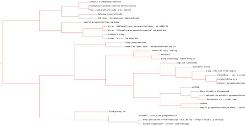
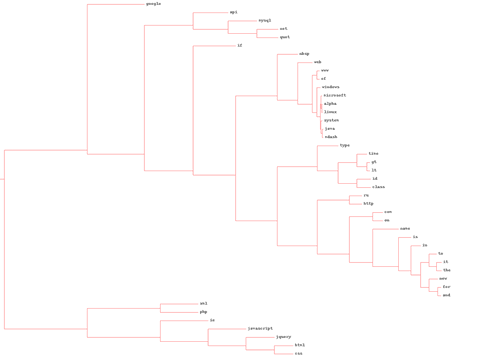
And here is the most interesting moment. As a result of the scripts, the following dendrograms were obtained:
1) for blogs (in full quality - img-fotki.yandex.ru/get/4100/serg-panarin.0/0_21f52_b8057f0d_-1-orig.jpg )
2) for words (in full quality - img-fotki.yandex.ru/get/4102/serg-panarin.0/0_21f53_dcdea04f_-1-orig.jpg )
By changing feedlist.txt you can analyze arbitrary blogs and get your dendrograms.
There was a desire in one post to consider cluster analysis, its beautiful implementation in Python, and, especially, the visual representation of clusters - dendrograms .
The code of the example is based on the code of the examples from the book.
')
The main idea of cluster analysis is the selection among a multitude of data groups within which the elements are to some extent similar. As part of this analysis, in fact, there is a certain classification of the studied data due to their distribution into groups. These groups are arranged hierarchically and the structure of the clusters that have been obtained after the analysis can be represented as a tree - dendrogram (“dendro”, as is well known, in Greek, “tree”).
The measure of similarity for each problem can be given its own, but the simplest are the Euclidean distance and the Pearson correlation coefficient . The example deals with the Pearson correlation coefficient, but it can be easily replaced.
In general, historically, cluster analysis became the most popular in the humanities, and one of the first tasks for which it was used was the analysis of data on ancient burials.
The cluster construction algorithm is, in principle, simple and logical.
The initial data for the algorithm is a list of some elements and a function of similarity between them (the "proximity" of elements). Each element has “coordinates” in a certain space (for example, in the space of numbers of words), by which the similarity between the elements is calculated.
Example: elements - blogs, 2 "coordinates" - the number of words "php" and "xml" in the content of blogs.
The blog number 1 - 7 times found the word "php" and 5 times "xml". Then the “coordinates” of the blog №1 in the space of the number of these words are (7; 5).
Blog # 2 has the word “php” 6 times and “xml” 4 times. Then the “coordinates” of the blog №2 in the space of the number of these words is (6; 4).
The similarity is determined by the function - Euclidean distance.
d(blog1, blog2) = sqrt( (7-6)^2 + (5-4)^2) = 1.414
At the output we get a tree of clusters (cluster hierarchy).
The algorithm works as follows:
1) Step 1: Count each element of the source list as a cluster and add them to the merge list
2) Step 2 - N: Find the closest clusters and merge them into a new one (the “coordinates” of the new - the half-sum of the “coordinates” being joined). Add a new union to the list , and remove original clusters from the list . Thus, at each step in the merge list, there are fewer elements.
Stop criterion : presence of only one cluster in the merge list , which can no longer be merged (getting one, “root” cluster)
This algorithm is implemented by the hcluster function:
* This source code was highlighted with Source Code Highlighter .
- def hcluster (rows, distance = pearson):
- distances = {}
- currentclustid = -1
- # Clusters are initially just the rows
- clust = [bicluster (rows [i], id = i) for i in range (len (rows))]
- while len (clust)> 1:
- lowestpair = (0,1)
- closest = distance (clust [0] .vec, clust [1] .vec)
- # loop through every distance
- for i in range (len (clust)):
- for j in range (i + 1, len (clust)):
- # distance is
- if (clust [i] .id, clust [j] .id) not in distances:
- distance [(clust [i] .id, clust [j] .id)] = distance (clust [i] .vec, clust [j] .vec)
- d = distances [(clust [i] .id, clust [j] .id)]
- if d <closest:
- closest = d
- lowestpair = (i, j)
- # calculate the average of the two clusters
- mergevec = [
- (clust [lowestpair [0]]. vec [i] + clust [lowestpair [1]]. vec [i]) / 2.0
- for i in range (len (clust [0] .vec))]
- # create the new cluster
- newcluster = bicluster (mergevec, left = clust [lowestpair [0]],
- right = clust [lowestpair [1]],
- distance = closest, id = currentclustid)
- # cluster ids that weren't in the original set are negative
- currentclustid- = 1
- del clust [lowestpair [1]]
- del clust [lowestpair [0]]
- clust.append (newcluster)
- return clust [0]
The example will be considered an example of cluster analysis of the contents of programming blogs. The book deals with English-language blogs, but I decided to analyze 35 Russian-language terms of English-speaking terms. To display the results of the analysis, the names of the blogs had to be translated using a small library.
The full archive with all the necessary files and scripts in Python can be downloaded - clusters.zip
The composition of the archive:
blogdata.txt –
clusters.py -
draw_dendrograms.py - ( clusters.py)
feedlist.txt - RSS
generatefeedvector.py - blogdata.txt

translit.py, utils.py -
feedlist.txt with a list of RSS blogs, you can take, for example, such content (taken from the search http://lenta.yandex.ru/feed_search.xml?text=programming ):
feeds.feedburner.com/nayjest
www.codenet.ru/export/read.xml
feeds2.feedburner.com/simplecoding
feeds2.feedburner.com/nickspring
feeds2.feedburner.com/Sribna
community.livejournal.com/ru_cpp/data/rss
community.livejournal.com/ru_lambda/data/rss
feeds2.feedburner.com/rusarticles
feeds2.feedburner.com/Jstoolbox
feeds2.feedburner.com/rsdn/cpp
4matic.wordpress.com/feed
www.nowa.cc/external.php?type=RSS2
www.gotdotnet.ru/blogs/gaidar/rss
community.livejournal.com/ru_programmers/data/rss
www.compdoc.ru/rssdok.php
feeds2.feedburner.com/rsdn/philosophy
softwaremaniacs.org/blog/feed
community.livejournal.com/new_ru_php/data/rss
www.newsrss.ru/mein_rss/rss_cdata.xml
feeds2.feedburner.com/5an
subscribe.ru/archive/comp.soft.prog.linuxp/index.rss
feeds.feedburner.com/mrkto
rbogatyrev.livejournal.com/data/rss
feeds2.feedburner.com/poisonsblog
community.livejournal.com/ruby_ru/data/rss
feeds2.feedburner.com/devoid
rgt.rpod.ru/rss.xml
feeds2.feedburner.com/rsdn/decl
feeds2.feedburner.com/Toeveryonethe
www.osp.ru/rss/Software.rss
feeds2.feedburner.com/Freshcoder
blogs.technet.com/craftsmans_notes/rss.xml
feeds2.feedburner.com/RuRubyRails
feeds2.feedburner.com/bitby
opita.net/rss.xml
The program for constructing dendrograms itself consists of 2 scripts (data collection + processing), which are launched sequentially:
python generatefeedvector.py

python draw_dengrograms.py
The example will require a Python Imaging Library (PIL), which can be downloaded from www.pythonware.com/products/pil
After unzipping, it is installed as usual:
python setup.py installAnd here is the most interesting moment. As a result of the scripts, the following dendrograms were obtained:
1) for blogs (in full quality - img-fotki.yandex.ru/get/4100/serg-panarin.0/0_21f52_b8057f0d_-1-orig.jpg )
2) for words (in full quality - img-fotki.yandex.ru/get/4102/serg-panarin.0/0_21f53_dcdea04f_-1-orig.jpg )
By changing feedlist.txt you can analyze arbitrary blogs and get your dendrograms.
Source: https://habr.com/ru/post/79756/
All Articles