Image recognition. Algorithm Eigenface

Introduction

I continue a series of articles on pattern recognition, computer vision and machine learning. Today I present to you an overview of the algorithm, which is called eigenface.





')

The algorithm is based on the use of fundamental statistical characteristics: averages ( mat. Expectation ) and covariance matrix ; using the principal component method . We will also touch upon such concepts of linear algebra as eigenvalues ​​(eigenvalues) and eigenvectors (eigenvectors) (wiki: ru , eng ). And in addition, we will work in multidimensional space.

No matter how scary it all sounds, this algorithm is probably one of the simplest ones I have examined, its implementation does not exceed several dozen lines, at the same time it shows quite good results in a number of tasks.





For me, eigenface is interesting because for the last 1.5 years I have been developing, including statistical algorithms for processing various data arrays, where very often we have to deal with all the above “pieces”.

Tools

According to the current methodology, after thinking about an algorithm, but before implementing it in C / C ++ / C # / Python etc., it is necessary to quickly (as far as possible) create a mathematical model and test it, count something. This allows you to make the necessary adjustments, correct errors, to detect what was not taken into account when thinking about the algorithm. For all this I use MathCAD . The advantage of MathCAD is that along with a huge number of built-in functions and procedures, it uses classical mathematical notation. Roughly speaking, it is enough to know mathematics and be able to write formulas.

Brief description of the algorithm

Like any algorithm from the machine learning series, the eigenface must first be trained; for this, a training set is used, which is an image of the people we want to recognize. After the model is trained, we will submit some image to the input and as a result we will get an answer to the question: which image from the training set most likely corresponds to an example at the input, or does not correspond to any.



The task of the algorithm is to present the image as the sum of the basis components (images):





Where Φ _i is the centered (i.e. minus the average) i-th image of the original sample, w _j are weights and u _{j are} eigenvectors (eigenvectors or, within this algorithm, eigenfaces).







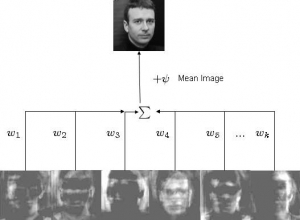
In the picture above, we get the original image by weighted summation of the eigenvectors and by adding the average. Those. with w and u, we can restore any original image.



The training set needs to be projected into a new space (and the space, as a rule, is much more dimension than the original 2-dimensional image), where each dimension will make a certain contribution to the overall presentation. The method of principal components allows one to find a basis for a new space so that the data in it are located, in a sense, optimally. To understand, just imagine that in the new space some dimensions (aka main components or eigenvectors or eigenfaces) will “carry” more general information, while others will only carry specific information. As a rule, higher-order dimensions (corresponding to smaller eigenvalues) carry much less useful (in our case, useful means something that gives a generalized view of the whole sample) information than the first dimensions corresponding to the largest eigenvalues. Leaving the dimensions with only useful information, we obtain a feature space in which each image of the original sample is represented in a generalized form. This is very simplistic, and the idea of ​​the algorithm consists.

Further, having on hand some image, we can map it to the space created in advance and determine to which image of the training set our example is located the closest. If it is located at a relatively large distance from all data, then this image with a high probability does not belong to our database at all.



For a more detailed description, I advise you to refer to the list of External links on Wikipedia.



A small digression. The method of principal components is quite widespread. For example, in my work I use it to select components of a certain scale (temporal or spatial), direction or frequency in an array of data. It can be used as a method for data compression or a method for reducing the original dimension of a multidimensional sample.

Creating a model

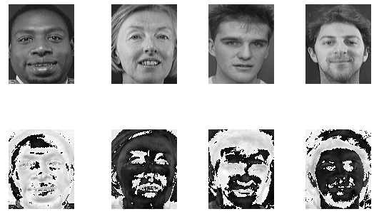
The Olivetti Research Lab's (ORL) Face Database was used to compile the training sample. There are 10 photos of 40 different people:





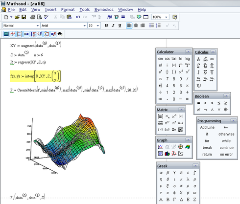
To describe the implementation of the algorithm, I will insert here screenshots with functions and expressions from MathCAD and comment on them. Go.



one.







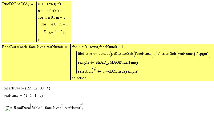
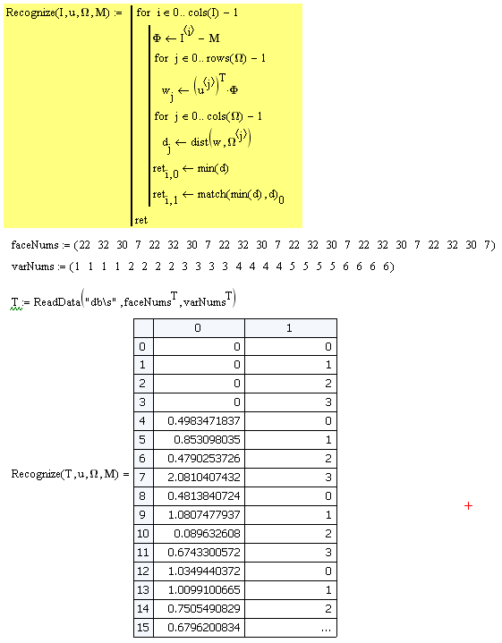
faceNums sets the vector of numbers of persons to be used in training. varNums sets the version number (according to the database description, we have 40 directories each with 10 image files of the same person). Our training sample consists of 4 images.

Next, we call the ReadData function. It implements sequential data reading and image transfer to a vector (TwoD2OneD function):







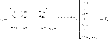
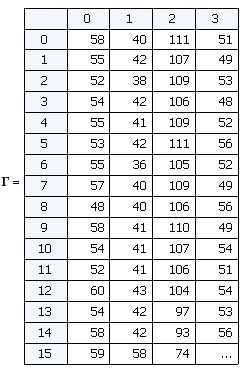
Thus, at the output we have a matrix Γ, each column of which is an image “expanded” into a vector. Such a vector can be considered as a point in multidimensional space, where the dimension is determined by the number of pixels. In our case, images with a size of 92x112 give a vector of 10304 elements or set a point in 10304-dimensional space.







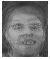
2. It is necessary to normalize all the images in the training set, taking away the average image. This is done in order to leave only unique information, removing the elements common to all images.







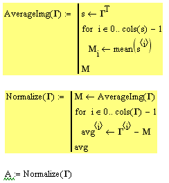
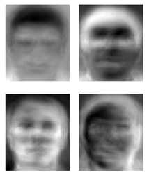
The AverageImg function counts and returns the mean vector. If we “turn” this vector into an image, we will see “averaged face”:







The Normalize function subtracts the average vector from each image and returns the average sample:







3. The next step is the calculation of eigenvectors (they are also eigenfaces) u and weights w for each image in the training sample. In other words, it is a transition to a new space.







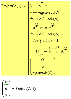
We calculate the covariance matrix, then we find the main components (they are also eigenvectors) and count the weights. Those who are closer to the algorithm will enter the mathematics. The function returns the weights matrix, eigenvectors and eigenvalues. These are all necessary to display data in a new space. In our case, we work with 4-dimensional space, by the number of elements in the training sample, the remaining 10304 - 4 = 10300 dimensions are degenerate, we do not take them into account.



We, on the whole, do not need eigenvalues, but we can trace some useful information from them. Let's take a look at them:







The eigenvalues ​​actually show the dispersion along each of the axes of the principal components (each component corresponds to one dimension in space). Look at the right expression, the sum of this vector = 1, and each element shows the contribution to the total variance of the data. We see that 1 and 3 main components give a total of 0.82. Those. 1 and 3 dimensions contain 82% of all information. The second dimension is collapsed, and the fourth carries 18% of the information and we do not need it.

Recognition

The model is made up. We will test.







We are creating a new sample of 24 items. The first 4 elements of the element are the same as in the training sample. The rest are different versions of the images from the training sample:







Next, load the data and transfer it to the Recognize procedure. In it, each image is averaged, displayed in the space of the main components, weights w are. After the vector w is known, it is necessary to determine which of the existing objects it is closest to. For this, the dist function is used (instead of the classical Euclidean distance in pattern recognition problems, it is better to use another metric: Mahalanobis distance ). The minimum distance and the index of the object to which this image is located closest.



On a sample of 24 objects shown above, the efficiency of the classifier is 100%. But there is one nuance. If we submit an image to the input that is not in the original database, then the vector w will still be calculated and the minimum distance will be found. Therefore, the criterion O is introduced, if the minimum distance <O means the image belongs to the class of recognizable, if the minimum distance is> O, then there is no such image in the database. The value of this criterion is chosen empirically. For this model, I chose O = 2.2.



Let's make a sample of people who are not in the training and see how effectively the classifier will eliminate false samples.







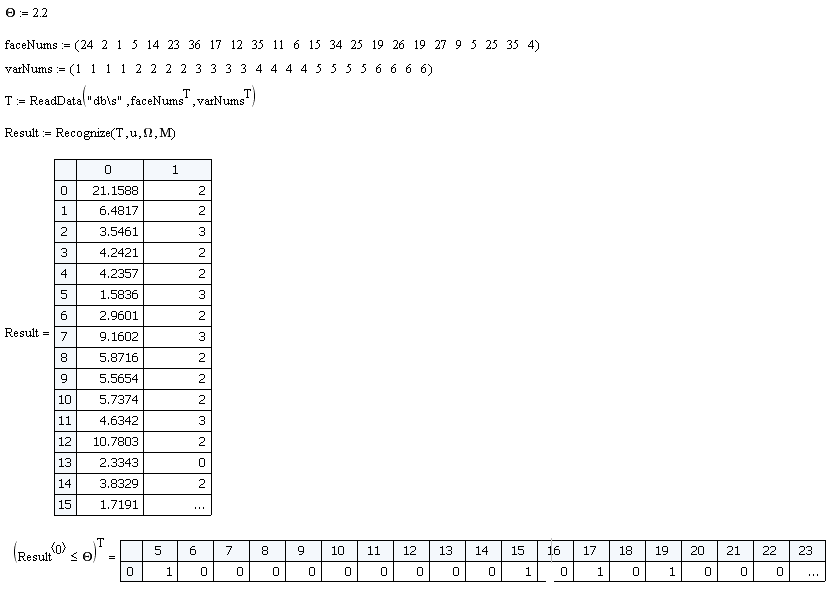
Of the 24 samples, we have 4 false positives. Those. efficiency was 83%.

Conclusion

In general, a simple and original algorithm. Once again, he proves that in spaces of higher dimension there is a “hidden” set of useful information that can be used in various ways.  Coupled with other advanced techniques, eigenface can be used to improve the efficiency of solving tasks.



For example, we use a simple distance classifier as a classifier. However, we could apply a more advanced classification algorithm, for example, the Support Vector Machine or the neural network.



The next article focuses on the Support Vector Machine. A relatively new and very interesting algorithm, in many problems it can be used as an alternative to NA.



When writing the article materials were used:

onionesquereality.wordpress.com

www.cognotics.com



Materials:

Calculation sheet for MathCAD 14



UPD:

I see many incomprehensible and frightened mathematics. There are two ways.

1. If you want to understand the whole point of all the actions of the algorithm, then you should start by understanding the basic things: Cove. matrices, the method of principal components, the meaning and meaning of eigenvectors and values. If you know what it is, then everything becomes clear.

2. If you want to simply implement and use the algorithm, then take the list of calculations for MathCAD'a. Run, look, change the parameters. There are calculations on the floor of the screen and there is nothing more difficult in them than multiplying matrices (well, except for the built-in functions for calculating eigenvectors, but it is not necessary to delve into this). This is to help with the implementation in python , matlab , C ++ .