Intro

With this article I begin a cycle of articles about well-known and not-so data structures as well as their application in practice.

In my articles I will give examples of code in two languages ​​at once: in Java and in Haskell. Thanks to this, it will be possible to compare the imperative and functional styles of programming and see the pros and cons of both.
')
I decided to start with binary search trees, as this is a fairly basic, but at the same time interesting thing, which also has a large number of modifications and variations, as well as practical applications.

Why do you need it?

Binary search trees are usually used to implement sets and associative arrays (for example, set and map in c ++ or TreeSet and TreeMap in java). More complex applications include ropes (I will talk about them in one of the following articles), various algorithms of computational geometry, mainly in algorithms based on the “scanning straight line”.

In this article, trees will be considered on the example of the implementation of an associative array. An associative array is a generalized array in which indices (usually called keys) can be arbitrary.

Well, let's get started

A binary tree consists of vertices and links between them. More specifically, the tree has a distinguished vertex-root and each vertex can have left and right sons. In words it sounds somewhat difficult, but if you look at the picture, everything becomes clear:



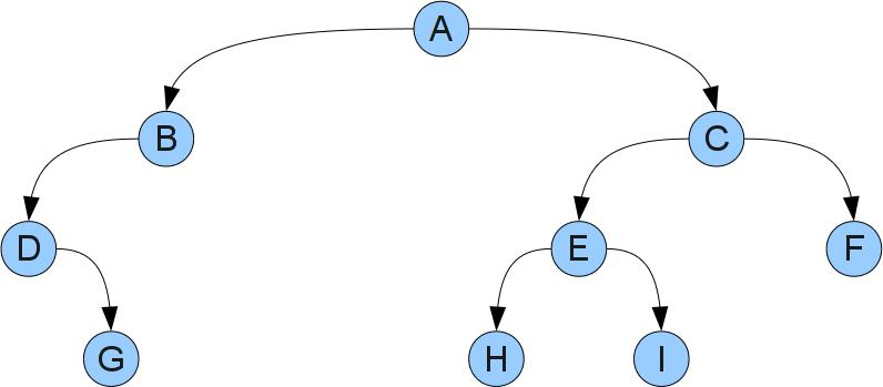
In this tree, root will be A. It can be seen that D has no left son, D has right, and B, and G, H, F, and I have both. Peaks without sons are called leaves.

Each vertex X can be associated with its own tree, consisting of the vertex, its sons, the sons of its sons, etc. Such a tree is called a subtree with a root X. Left and right subtrees of X are called subtrees with roots in the left and right sons of X, respectively. Note that such subtrees may be empty if X does not have a corresponding son.

The data in the tree is stored at its vertices. In programs, tree tops are usually represented by a structure storing data and two references to the left and right son. Missing vertices are null or special Leaf constructor:

data Ord key => BSTree key value = Leaf | Branch key value (BSTree key value) (BSTree key value) deriving (Show) 

 static class Node<T1, T2> { T1 key; T2 value; Node<T1, T2> left, right; Node(T1 key, T2 value) { this.key = key; this.value = value; } } 

As you can see from the examples, we require from the keys that they can be compared with each other ( Ord a in haskell and T1 implements Comparable<T1> in java). All this is not casual - in order for the tree to be useful data must be stored in it according to some rules.

What are these rules? Everything is simple: if the key x is stored in the vertex X, then in the left (right) subtree only keys smaller (correspondingly larger) than x should be stored. Illustrate:



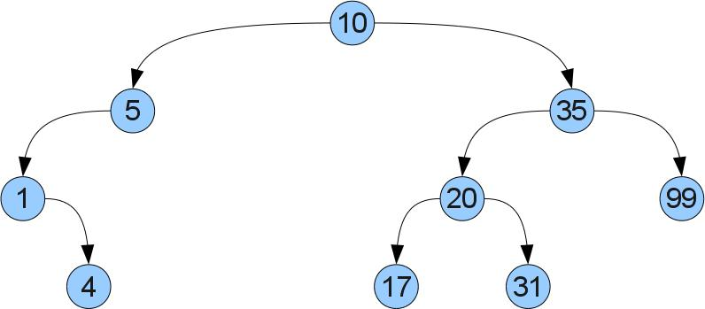
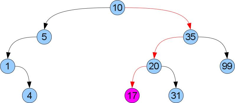
What gives us such ordering? That we can easily find the required key x in the tree! Just compare x with the value at the root. If they are equal, then we have found the required. If x is less (more), then it can only be in the left (respectively right) subtree. Let for example we look for the number 17 in a tree:



The function that receives the value by key:

 get :: Ord key => BSTree key value -> key -> Maybe value get Leaf _ = Nothing get (Branch key value left right) k | k < key = get left k | k > key = get right k | k == key = Just value 

 public T2 get(T1 k) { Node<T1, T2> x = root; while (x != null) { int cmp = k.compareTo(x.key); if (cmp == 0) { return x.value; } if (cmp < 0) { x = x.left; } else { x = x.right; } } return null; } 

Add to tree

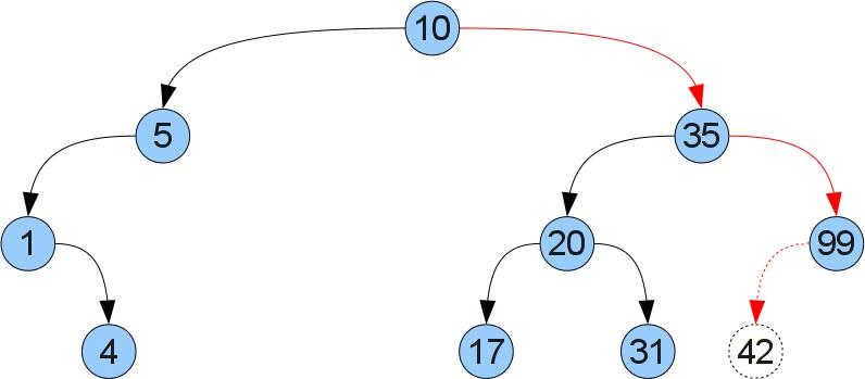
Now let's try the operation of adding a new key / value pair (a, b). To do this, we will descend the tree as in the get function until we find a vertex with the same key, or we reach the missing son. If we find a vertex with the same key, then simply change the corresponding value. In the opposite case, it is easy to understand that it is in this place that a new vertex should be inserted in order not to disturb the order. Consider inserting key 42 into the tree in the past figure:



Code:

 add :: Ord key => BSTree key value -> key -> value -> BSTree key value add Leaf kv = Branch kv Leaf Leaf add (Branch key value left right) kv | k < key = Branch key value (add left kv) right | k > key = Branch key value left (add right kv) | k == key = Branch key value left right 

 public void add(T1 k, T2 v) { Node<T1, T2> x = root, y = null; while (x != null) { int cmp = k.compareTo(x.key); if (cmp == 0) { x.value = v; return; } else { y = x; if (cmp < 0) { x = x.left; } else { x = x.right; } } } Node<T1, T2> newNode = new Node<T1, T2>(k, v); if (y == null) { root = newNode; } else { if (k.compareTo(y.key) < 0) { y.left = newNode; } else { y.right = newNode; } } } 

Lyrical digression about the pros and cons of the functional approach

If you carefully consider the examples in both languages, you can see some differences in the behavior of functional and imperative implementations: if java we simply modify the data and references in the existing vertices, the version of haskell creates new vertices along the entire path traversed by recursion. This is due to the fact that destructive assignments cannot be made in purely functional languages. Clearly, this degrades performance and increases memory consumption. On the other hand, such an approach also has positive aspects: the absence of side effects greatly facilitates the understanding of how the program functions. In more detail about it it is possible to read in almost any textbook or introductory article about functional programming.

In this article, I want to draw attention to another consequence of the functional approach: even after adding a new element to the tree, the old version will remain available! Due to this effect, ropes work, including in the implementation in imperative languages, allowing you to implement strings with asymptotically faster operations than with the traditional approach. I will tell you about ropes in one of the following articles.

Back to our sheep

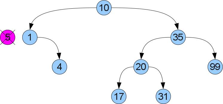
Now we are getting close to the most difficult operation in this article - removing the key x from the tree. To begin with, we, as before, will find our top in the tree. Now there are two cases. Case 1 (delete the number 5):



It can be seen that the deleted vertex has no right son. Then we can remove it and insert the left subtree instead of it, without disturbing the order:



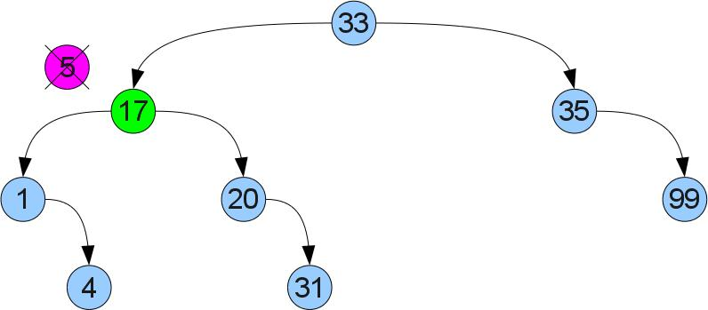
If the right-hand son is, case 2 is present (we delete the top 5 again, but from a slightly different tree):



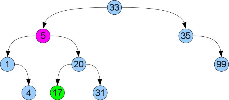
It will not be so easy here - the left son may already have a right son. We proceed differently: we find the minimum in the right subtree. It is clear that you can find it if you start in the right son and go all the way to the left. Since the found minimum does not have a left son, you can cut it out by analogy with case 1 and insert it in place of the removed vertex. Due to the fact that it was minimal in the right subtree, the order property will not be broken:



Implementing removal:

 remove :: Ord key => BSTree key value -> key -> BSTree key value remove Leaf _ = Leaf remove (Branch key value left right) k | k < key = Branch key value (remove left k) right | k > key = Branch key value left (remove right k) | k == key = if isLeaf right then left else Branch leftmostA leftmostB left right' where isLeaf Leaf = True isLeaf _ = False ((leftmostA, leftmostB), right') = deleteLeftmost right deleteLeftmost (Branch key value Leaf right) = ((key, value), right) deleteLeftmost (Branch key value left right) = (pair, Branch key value left' right) where (pair, left') = deleteLeftmost left 

 public void remove(T1 k) { Node<T1, T2> x = root, y = null; while (x != null) { int cmp = k.compareTo(x.key); if (cmp == 0) { break; } else { y = x; if (cmp < 0) { x = x.left; } else { x = x.right; } } } if (x == null) { return; } if (x.right == null) { if (y == null) { root = x.left; } else { if (x == y.left) { y.left = x.left; } else { y.right = x.left; } } } else { Node<T1, T2> leftMost = x.right; y = null; while (leftMost.left != null) { y = leftMost; leftMost = leftMost.left; } if (y != null) { y.left = leftMost.right; } else { x.right = leftMost.right; } x.key = leftMost.key; x.value = leftMost.value; } } 

For dessert, a couple of features that I used to test:

 fromList :: Ord key => [(key, value)] -> BSTree key value fromList = foldr (\(key, value) tree -> add tree key value) Leaf toList :: Ord key => BSTree key value -> [(key, value)] toList tree = toList' tree [] where toList' Leaf list = list toList' (Branch key value left right) list = toList' left ((key, value):(toList' left list)) 

Why is all this useful?

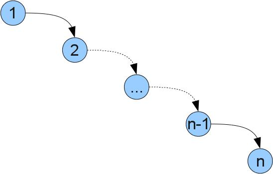
The reader may wonder why such difficulties are needed if you can simply store a list of pairs [(key, value)]. The answer is simple - tree operations work faster. When implemented in a list, all functions require O (n) actions, where n is the size of the structure. (Writing O (f (n)) roughly means “proportional to f (n)”, a more correct description and details can be read here ). Tree operations work in O (h), where h is the maximum depth of the tree (depth is the distance from the root to the top). In the optimal case, when the depth of all leaves is the same, there will be n = 2 ^ h vertices in the tree. Therefore, the complexity of operations in trees close to optimum will be O (log (n)). Unfortunately, in the worst case, the tree may degenerate and the complexity of the operations will be as in the list, for example in such a tree (you can, if you insert the numbers 1..n in order):



Fortunately, there are ways to implement a tree so that the optimal depth of the tree is maintained for any sequence of operations. Such trees are called balanced. These include red-black trees, AVL trees, splay trees, etc.

The announcement of the next series

In the next article I will make a small overview of various balanced trees, their pros and cons. In the following articles I will talk about some (possibly several) in more detail and with the implementation. After that I will talk about the implementation of ropes and other possible extensions and applications of balanced trees.

Stay in touch!

useful links

Sources of examples entirely:

on haskell

on java

Wikipedia article

Interactive BST Operations Visualizer

I also strongly advise reading the book by Kormen T., Leiserson Ch., Rivest R .: “Algorithms: construction and analysis”, which is an excellent textbook on algorithms and data structures

UPD: pictures restored, thanks Xfrid !