Introduction

As it turned out, the topic of algorithms is interesting for the Habra community. Therefore, as promised, I will begin a series of reviews of “classical” algorithms on graphs.

Since the audience at Habré is different, and the topic is interesting to many, I have to start from the zero part. In this part I will tell you what a graph is, how it is presented in a computer and why it is used. I apologize in advance to those who already know this very well, but in order to explain the algorithms on graphs, you must first explain what a graph is. Without this in any way.

The basics

In mathematics, a graph is an abstract representation of a set of objects and the connections between them. A graph is a pair of (V, E) where V is a set of vertices , and E is a set of pairs, each of which is a link (these pairs are called edges ).

The graph can be oriented or unoriented . In a directed graph, links are directed (that is, the pairs in E are ordered, for example, the pairs (a, b) and (b, a) are two different links). In turn, in an undirected graph, the links are undirected, and therefore if there is a connection (a, b), then it means that there is a connection (b, a).





')

Example:

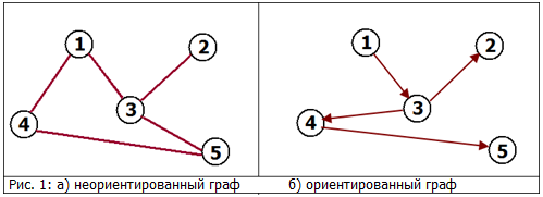
Undirected graph: Neighborhood (in life). If (1) neighbor (3), then (3) neighbor (1). See fig. 1.a



Oriented graph: Links. The site (1) may refer to the site (3), but it is not at all necessary (although possible) that the site (3) refers to the site (1). See fig. 1.b

The degree of the vertex can be incoming and outgoing (for undirected graphs, the incoming degree is equal to outgoing).

The incoming degree of a vertex v is the number of edges of the form (i, v ), that is, the number of edges that “enter” into v.

The outgoing degree of a vertex v is the number of edges of the form ( v , i), that is, the number of edges that "go out" of v.

This is not a completely formal definition (more formally a definition through incidence ), but it fully reflects the essence



The path in the graph is a finite sequence of vertices, in which every two vertices reaching in a row are connected by an edge. The path can be oriented or undirected depending on the graph. In Figure 1.a, the path is for example the sequence [(1), (4), (5)] in Figure 1.b, [(1), (3), (4), (5)].



There are many other properties of graphs (for example, they may be connected, dicotyledonous, complete), but I will not describe all these properties now, and in the following parts when we need these concepts.

Graph representation

There are two ways to represent a graph, as adjacency lists and as an adjacency matrix. Both methods are suitable for representing directed and undirected graphs.



Adjacency matrix

This method is convenient for representing dense graphs in which the number of edges (| E |) is approximately equal to the number of vertices in the square (| V | ² ).

In this view, we fill in a matrix of size | V | x | V | as follows:

A [i] [j] = 1 (If there is an edge from i to j)

A [i] [j] = 0 (Else)

This method is suitable for oriented and undirected graphs. For undirected graphs, the matrix A is symmetric (that is, A [i] [j] == A [j] [i], because if there is an edge between i and j, then it is also an edge from i to j, and edge from j to i). Thanks to this property, it is possible to reduce the memory usage almost by half, keeping the elements only in the upper part of the matrix, above the main diagonal)

It is clear that using this representation method, you can quickly check if there is an edge between the vertices v and u, simply by looking at the cell A [v] [u].

On the other hand, this method is very cumbersome, since it requires O (| V | ² ) memory to store the matrix.





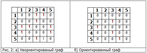
In fig. 2 shows the graph representations from Fig. 1 using adjacency matrices.



Adjacency lists

This presentation method is more suitable for sparse graphs, that is, graphs whose number of edges is much less than the number of vertices in the square (| E | << | V | ² ).

This view uses the array Adj containing | V | lists. Each Adj [v] list contains all vertices of u, so there is an edge between v and u. The memory required for representation is O (| E | + | V |), which is a better indicator than the adjacency matrix for sparse graphs.

The main disadvantage of this method of representation is that there is no quick way to check whether the edge (u, v) exists.







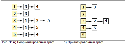
In fig. 3 shows the graph representations from Fig. 1 using adjacency lists.

Application

Those who read up to this place, probably asked themselves the question, and where exactly can I apply the graphs. As I promised, I will try to give examples. The very first example that comes to mind is a social network. The vertices of the graph are people, and the edges of the relationship (friendship). The count can be undirected, that is, I can be friends only with those who are friends with me. Or oriented (like for example in LiveJournal), where you can add a person as a friend, without him adding you. If he adds you, you will be “mutual friends.” That is, there will be two edges: (He, you) and (You, He)

Another of the applications of the graph, which I have already mentioned is links from site to site. Imagine you want to make a search engine and want to consider which sites have more links (for example, site A), while taking into account how many sites link to site B, which links to site A. You will have an adjacency matrix of these links. You will want to introduce some sort of rating calculation system that does some sort of calculation on this matrix, well, then ... it's Google (more precisely, PageRank) =)

Conclusion

This is a small part of the theory that we need for the following parts. I hope you understand, and most importantly, I like it and are interested in reading further parts! Leave your comments and suggestions in the comments.

In the next part

BFS - search algorithm in width

Bibliography

Kormen, Lizerson, Riverst, Stein - Algorithms. Construction and analysis. Williams Publishing, 2007.

Glossary of graph theory

Count - an article in the English Wikipedia



The article is a cross-post from my blog - " Programing as is - notes programmer"



______________________

Text prepared in the Habr Editor