Vector graphics in LaTeX. PGF / TikZ package

Good day. I have long been going to talk about the possibilities of vector graphics in LaTeX provided by the low-level macro package PGF and its extension TikZ, and the release of the previous article on the Xy-pic package for creating diagrams and graphs and the appearance of free time made it possible to start working :-).

I once needed to find and study some kind of flexible means for creating high-quality vector images, because they already got crookedly scaled, inserted with a terrible extension of the image of raster formats, spoiling the whole impression of the document, and doubling its size for one big picture with a rectangle and several captions to it. The available capabilities of the built-in picture environment are very scarce; PStricks is focused on PostScript (it doesn't work with pdflatex, which I need), although it can do something that PGF cannot; The MetaPost system is perhaps the most powerful of all in this area, but it operates using a separate interpreter with all the ensuing consequences. Thus, the choice fell on PGF / TikZ .



The main purpose of this article is the presence of a sufficient number of links and a small number of examples with a description in Russian. This is in most cases enough to understand whether you need it or not.
')
It is very nice when for some tool there is an exhaustive list of examples of what it can do and how to achieve it. For the package under discussion, this list can be viewed by typing in the search engine "pgf examples" and clicking on the first link. Here are all the examples in one list: www.texample.net/tikz/examples/all . There is no point in trying to describe everything the package is capable of. Perhaps, I will focus on the basic concepts.

The article discusses the use of pgf / tikz with the macro package LaTeX, as the most common, but pgf / tikz also works with others. The text of the article is based mainly on the manual TikZ & PGF. Manual for Version 2.00 (560 p.). Some examples are taken from it. Also in the book there is a small, but useful chapter Guidelines on Graphics (p. 65), devoted to the general principles of working on documents with vector graphics, including examples of how to do it and how not to do it; it is worth referring to it regardless of whether you will use pgf / tikz or something else later.

Installation

On GNU / Linux, you need to install the pgf package (and the dependent xcolor version> = 2.00). If this is not the case, it is enough to unzip the source (locally or globally) and make a texhash (see the manual for details). In Windows, pgf / tikz is included in the MiKTeX distribution, so no additional installation is required.

Broadcast

For pdf use

pdflatex file.tex


To get ps, we use two commands:

latex file.tex
dvips file.dvi


Also interesting is the ability to convert to HTML and SVG.

Using

To use the basic features of the package, you must connect it in the preamble with the command

\usepackage { tikz }


To insert pgf / tikz commands, use either the \tikz with one argument (usually to insert a picture within a string), or the \begin[ options ]{tikzpicture}...\end{tikzpicture} . If you need to specify several drawing commands in the argument to \tikz , they are surrounded by curly braces ( \tikz[ options ]{...} ). Each command ends with a semicolon.

\documentclass { memoir } <br>
\pagestyle { empty } <br>
\usepackage { tikz } <br>
<br>
\begin{document} <br>
\tikz { \draw (-1,-1) -- (1,1); \path [ fill=green!80!blue,draw=red ] (0,0) circle ( 7mm ); } <br>
\end{document}


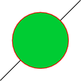
It is very convenient that you do not need to specify the size of the canvas. The program itself will calculate it for you.

Points

Points are set absolutely or relatively. Examples of Cartesian and polar coordinates:

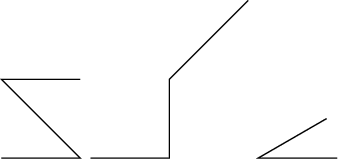
• (2,0) - point with given coordinates in current units (by default - 1 cm);
• (2cm,-3pt) - 2 cm in the direction of Ox, –3 points in the direction of Oy;
• (30:5cm) - a point at a distance of 5 cm from the current position in the direction of 30 degrees;
• +(2,0) - point separated from the current position by 2 units to the right (the current position does not change);
• ++(2,0) - point separated from the current position by 2 units to the right, which becomes the new current position.

\tikz \draw (0,0) -- +(1,0) -- +(0,1) -- +(1,1);<br>
\tikz \draw (0,0) -- ++(1,0) -- ++(0,1) -- ++(1,1);<br>
\tikz \draw (1,0) -- (0,0) -- (30:1);


Barycentric coordinates, a coordinate system of nodes (see below), a tangential system can also be used.

The coordinate system of intersections allows you to operate with the coordinates of the intersection (however, so far only for combinations of lines and circles). For this, the first and second objects (or their coordinates) and the intersection number (when there are several) are specified.

\begin { tikzpicture } <br>
\draw [ help lines ] (0,0) grid (3,2);<br>
\draw (0,0) coordinate (A) -- (3,2) coordinate (B)<br>
(1,2) -- (3,0);<br>
\fill [ red ] (intersection of A--B and 1,2--3,0) circle ( 2pt );<br>
\end { tikzpicture }


Coordinates can be specified using relative or absolute length modifiers or projections. This is done in the following ways:

• coordinate !number! angle: second_coordinate
• coordinate !dimension! angle: second_coordinate
• coordinate !projection_coordinate! angle: second_coordinate

For example,

• (1,2)!.25!(3,4) means a coordinate that is one quarter of the way from (1.2) to (3.4)
• (1,2)!1cm!(3,4) means a coordinate that is at a distance of 1 cm from the point (1.2) on the straight line (1.2) - (3.4)
• (1,2)!(0,5)!(3,4) means the coordinate, which is the projection of a point (0,5) onto a straight line (1,2) - (3,4)

Trajectories

A trajectory is a sequence of straight and curved lines. They are created using the \path command. If it is called without arguments, nothing will be drawn, which is not very interesting. Arguments can be draw , fill , shade , clip or any combination of them. Instead of \path[draw] , \path[fill] , \path[shade,draw] , ... you can use the abbreviations \draw , \fill , \shadedraw .

The basic command for creating lines is (a) -- (b) , where (a) and (b) are some points.

The cubic Bezier curve is given by the command (a) .. controls (x) and (y) .. (b) , where (a) and (b) are some points, (x) and (y) are anchor points that affect the shape crooked. If the and (y) skipped, it is considered that (y) = (x) .

Graphic parameters

They are specified in square brackets (as optional arguments in LaTeX) in the form of key-value sets: key=value . For example, \tikz \draw[line width=2pt,color=red] (1,0) -- (0,0) -- (1,0) -- cycle; . Sometimes the key= part can be omitted if the key for a given value is interpreted unambiguously.

Knots

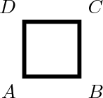
Text and captions are added to the picture as nodes. They are tied to the current position on the plane (in space), or explicitly tied to a certain point. As parameters, you can specify the anchor of the node binding (where it will be relative to the point: right, left, right above, etc.), the shape of the node (circle, square, ellipse, ...), the way it is displayed (draw, fill) other.

\tikz \draw (1,1) node { text } -- (2,2);


\begin { tikzpicture }[ line width=2pt ] <br>
\draw (0,0) node [ below left ] {$ A $} -- <br>
(1,0) node [ below right ] {$ B $} -- <br>
(1,1) node [ above right ] {$ C $} -- <br>
(0,1) node [ above left ] {$ D $} -- <br>
cycle;<br>
\end { tikzpicture }


Scopes

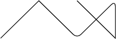
Using the scope environment, you can create scopes with your own parameters; the rest are inherited from the containing data. In fact, the tikzpicture environment behaves like a scope . With certain limitations, the scope can also be applied when drawing a path.

\tikz \draw (0,0) -- (1,1)<br>
{[ rounded corners ] -- (2,0) -- (3,1) } -- <br>
(3,0) -- (2,1);


Styles

Styles are specified when listing graphic parameters. There is a set of already defined ones that can be overridden. You can define your own.

\begin { tikzpicture }[ scale=0.7 ] <br>
\draw (0,0) grid +(2,2);<br>
\draw [ help lines ] (3,0) grid +(2,2);<br>
\end { tikzpicture }


Calculations

When connecting the calc library with the command in the preamble

\usetikzlibrary { calc }


You can use some mathematical calculations to determine the coordinates, for example,

\begin { tikzpicture }[ scale=0.5 ] <br>
\draw [ help lines ] (0,0) grid (4,3);<br>
\fill [ red ] ( $ 2*(1,1) $ ) circle ( 2pt );<br>
\fill [ green ] ( ${ 1+1 } *(1,.5) $ ) circle ( 2pt );<br>
\fill [ blue ] ( $ cos(0)*sin(90)*(1,1) $ ) circle ( 2pt );<br>
\fill [ black ] ( ${ 3*(4-3) } *(1,0.5) $ ) circle ( 2pt );<br>
\end { tikzpicture }


Conclusion

The package’s possibilities can be listed for a very long time (for example, I didn’t mention anything about graphs, trees and chains), but such an enumeration is not the case in one article, especially since there is the aforementioned site and an excellent guide with comprehensive examples of using each pgf / goodies package. tikz. To use it or not - you decide. I have been working with him for less than six months (and I didn’t know about him much earlier), but I already use it actively and have no regrets; in many cases, he greatly saved time and effort. If people have an interest, the story can be continued ;-)

Ps.
Images were made like this:

 $ latex qq.tex && dvips -K -o qq.ps qq.dvi && convert -antialias -seed 0 -density 200 -trim qq.ps qq.png

The backlight was exported from gvim ( emacs theme).