Monte Carlo Integration Application in Rendering
We all studied numerical methods in the course of mathematics. These are methods such as integration, interpolation, series, and so on. There are two types of numerical methods: deterministic and randomized.
Typical deterministic function integration function in the range It looks like this: we take evenly spaced points calculate at midpoint of each of the intervals defined by these points, summarize the results and multiply by the width of each interval . For sufficiently continuous functions with increasing the result will converge to the correct value.

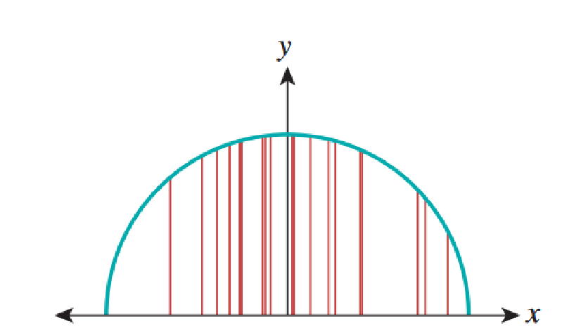
The probabilistic method, or the Monte Carlo method for calculating, or, more precisely, an approximate estimate of the integral in the range looks like this: let - randomly selected points in the interval . Then Is a random value whose average is an integral . To implement the method, we use a random number generator that generates points in the interval we calculate in each , average the results and multiply by . This gives us the approximate value of the integral, as shown in the figure below. with 20 samples approximates the correct result equal to .
')

Of course, every time we calculate such an approximate value, we will get a different result. The variance of these values depends on the shape of the function. . If we generate random points unevenly, then we need to slightly change the formula. But thanks to the use of uneven distribution of points, we get a huge advantage: forcing uneven distribution to give preference to points where large, we can significantly reduce the variance of the approximate values. This principle of non-uniform sampling is called sampling by significance .
Since over the past decades, a large-scale transition from deterministic to randomized approaches has taken place in rendering techniques, we will study the randomized approaches used to solve rendering equations. For this we use random variables, mathematical expectation and variance. We are dealing with discrete values, because computers are discrete in nature. Continuous quantities deal with the probability density function , but in the article we will not consider it. We’ll talk about the probability mass function. PMF has two properties:
The first property is called non-negativity. The second is called "normality." Intuitively, that represents the set of results of some experiment, and Is the result of probability member . The outcome is a subset of the probability space. The probability of an outcome is the sum of the PMF elements of this outcome, since
A random variable is a function, usually denoted by a capital letter, which sets real numbers in the probability space:
Note that the function - This is not a variable, but a function with real values. She is also not random , Is a separate real number for any result .
A random variable is used to determine outcomes. For example, many results , for which , that is, if ht and th are many lines denoting “eagles” or “tails,” then
and
it is an outcome with probability . We write it as . We use the predicate as a shortened entry for the outcome determined by the predicate.
Let's take a look at a piece of code simulating an experiment described by the formulas presented above:
Here we denote by
Now the analogy is becoming clearer. The many possible executions of a program and their associated probabilities are the probability space. Program variables that depend on
Let's discuss the expected value, also called the average. This is essentially the sum of the product of PMF and a random variable:
Imagine that h are “eagles” and t are “tails”. We have already covered ht and th. There are also hh and tt. Therefore, the expected value will be as follows:
You may wonder where it came from . Here I meant that we should assign meaning by yourself. In this case, we assigned h to 1, and t to 0. equals 2 because it contains 2 .
Let's talk about distribution. The probability distribution is a function that gives the probabilities of various outcomes of an event.
When we say that a random variable has a distribution then should indicate .
Scattering values accumulated around is called its dispersion and is defined as follows:
Where Is average .
called standard deviation . Random variables and are called independent if:
Important properties of independent random variables:
When I started with a story about probability, I compared continuous and discrete probabilities. We examined discrete probability. Now let's talk about the difference between continuous and discrete probabilities:
PDF Properties:
But if the distribution evenly , then the pdf is defined like this:

With continuous probability defined as follows:
Now compare the definitions of PMF and PDF:
In the case of continuous probability, random variables are better called random points . Because if Is the probability space, and displayed in a different space than then we should call random point , not a random variable. The concept of probability density is applicable here, because we can say that for any we have:

Now let's apply what we have learned to the sphere. The sphere has three coordinates: latitude, longitude, and complement of latitude. We use longitude and latitude addition only in , two-dimensional Cartesian coordinates applied to a random variable turn her into . We get the following detail:
We start with a uniform probability density at , or . Look at the uniform probability density formula above. For convenience, we will write .
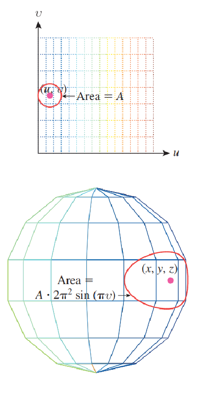
We have an intuitive understanding that if you select points evenly and randomly in a unit square and use to convert them to points on a unit sphere, they will accumulate next to the pole. This means that the obtained probability density in will not be uniform. This is shown in the figure below.
Now we will discuss ways to approximate the expected value of a continuous random variable and its application to determine the integrals. This is important because in rendering we need to determine the value of the reflectivity integral :
for various values and . Value Is the direction of the incident light. Code generating a random number uniformly distributed in the interval and taking the square root, creates a value in the range from 0 to 1. If we use PDF for it, since this is a uniform value, then the expected value will be equal . Also this value is the average value in this interval. What does this mean?
Consider Theorem 3.48 from the book Computer Graphics: Principles and Practice. She says that if is a function with real values, and is a uniform random variable in the interval then Is a random variable whose expected value has the form:
What does this tell us? This means that you can use a randomized algorithm to calculate the value of the integral if we execute the code many times and average the results .
In the general case, we get a certain value , as in the integral shown above, which needs to be determined, and some randomized algorithm that returns an approximate value . Such a random variable for a quantity is called an estimator . An estimator is considered to be distortion- free if its expected value is . In the general case, estimators without distortions are preferable to distortions.
We have already discussed discrete and continuous probabilities. But there is a third type, which is called mixed probabilities and is used in rendering. Such probabilities arise due to pulses in the distribution functions of bidirectional scattering, or pulses caused by point sources of illumination. Such probabilities are defined in a continuous set, for example, in the interval but not strictly defined by the PDF function. Consider the following program:
In sixty percent of the cases, the program will return 0.3, and in the remaining 40%, it will return a value evenly distributed in . The return value is a random variable with a probability mass of 0.6 at 0.3, and its PDF at all other points is specified as . We must define the pdf as:

In general, a mixed variable random variable is a variable for which there are a finite set of points in the PDF definition area, and vice versa, uniformly distributed points where the PMF is not defined.
Typical deterministic function integration function in the range It looks like this: we take evenly spaced points calculate at midpoint of each of the intervals defined by these points, summarize the results and multiply by the width of each interval . For sufficiently continuous functions with increasing the result will converge to the correct value.
The probabilistic method, or the Monte Carlo method for calculating, or, more precisely, an approximate estimate of the integral in the range looks like this: let - randomly selected points in the interval . Then Is a random value whose average is an integral . To implement the method, we use a random number generator that generates points in the interval we calculate in each , average the results and multiply by . This gives us the approximate value of the integral, as shown in the figure below. with 20 samples approximates the correct result equal to .
')
Of course, every time we calculate such an approximate value, we will get a different result. The variance of these values depends on the shape of the function. . If we generate random points unevenly, then we need to slightly change the formula. But thanks to the use of uneven distribution of points, we get a huge advantage: forcing uneven distribution to give preference to points where large, we can significantly reduce the variance of the approximate values. This principle of non-uniform sampling is called sampling by significance .
Since over the past decades, a large-scale transition from deterministic to randomized approaches has taken place in rendering techniques, we will study the randomized approaches used to solve rendering equations. For this we use random variables, mathematical expectation and variance. We are dealing with discrete values, because computers are discrete in nature. Continuous quantities deal with the probability density function , but in the article we will not consider it. We’ll talk about the probability mass function. PMF has two properties:
- For each exists .
The first property is called non-negativity. The second is called "normality." Intuitively, that represents the set of results of some experiment, and Is the result of probability member . The outcome is a subset of the probability space. The probability of an outcome is the sum of the PMF elements of this outcome, since
A random variable is a function, usually denoted by a capital letter, which sets real numbers in the probability space:
Note that the function - This is not a variable, but a function with real values. She is also not random , Is a separate real number for any result .
A random variable is used to determine outcomes. For example, many results , for which , that is, if ht and th are many lines denoting “eagles” or “tails,” then
and
it is an outcome with probability . We write it as . We use the predicate as a shortened entry for the outcome determined by the predicate.
Let's take a look at a piece of code simulating an experiment described by the formulas presented above:
headcount = 0 if (randb()): // first coin flip headcount++ if (randb()): // second coin flip headcount++ return headcount Here we denote by
ranb() Boolean function that returns true in half the cases. How is it related to our abstraction? Imagine a lot all possible executions of the program, declaring two executions the same values returned by ranb , pairwise identical. This means that there are four possible executions of the program in which two ranb() calls return TT, TF, FT, and FF. From our own experience, we can say that these four accomplishments are equally probable, that is, each occurs in about a quarter of cases.Now the analogy is becoming clearer. The many possible executions of a program and their associated probabilities are the probability space. Program variables that depend on
ranb calls are random variables. I hope you understand everything now.Let's discuss the expected value, also called the average. This is essentially the sum of the product of PMF and a random variable:
Imagine that h are “eagles” and t are “tails”. We have already covered ht and th. There are also hh and tt. Therefore, the expected value will be as follows:
You may wonder where it came from . Here I meant that we should assign meaning by yourself. In this case, we assigned h to 1, and t to 0. equals 2 because it contains 2 .
Let's talk about distribution. The probability distribution is a function that gives the probabilities of various outcomes of an event.
When we say that a random variable has a distribution then should indicate .
Scattering values accumulated around is called its dispersion and is defined as follows:
Where Is average .
called standard deviation . Random variables and are called independent if:
Important properties of independent random variables:
When I started with a story about probability, I compared continuous and discrete probabilities. We examined discrete probability. Now let's talk about the difference between continuous and discrete probabilities:
- Values are continuous. That is, the numbers are infinite.
- Some aspects of analysis require mathematical subtleties such as measurability .
- Our probability space will be infinite. Instead of PMF, we should use the probability density function (PDF).
PDF Properties:
- For each we have
But if the distribution evenly , then the pdf is defined like this:
With continuous probability defined as follows:
Now compare the definitions of PMF and PDF:
In the case of continuous probability, random variables are better called random points . Because if Is the probability space, and displayed in a different space than then we should call random point , not a random variable. The concept of probability density is applicable here, because we can say that for any we have:
Now let's apply what we have learned to the sphere. The sphere has three coordinates: latitude, longitude, and complement of latitude. We use longitude and latitude addition only in , two-dimensional Cartesian coordinates applied to a random variable turn her into . We get the following detail:
We start with a uniform probability density at , or . Look at the uniform probability density formula above. For convenience, we will write .
We have an intuitive understanding that if you select points evenly and randomly in a unit square and use to convert them to points on a unit sphere, they will accumulate next to the pole. This means that the obtained probability density in will not be uniform. This is shown in the figure below.
Now we will discuss ways to approximate the expected value of a continuous random variable and its application to determine the integrals. This is important because in rendering we need to determine the value of the reflectivity integral :
for various values and . Value Is the direction of the incident light. Code generating a random number uniformly distributed in the interval and taking the square root, creates a value in the range from 0 to 1. If we use PDF for it, since this is a uniform value, then the expected value will be equal . Also this value is the average value in this interval. What does this mean?
Consider Theorem 3.48 from the book Computer Graphics: Principles and Practice. She says that if is a function with real values, and is a uniform random variable in the interval then Is a random variable whose expected value has the form:
What does this tell us? This means that you can use a randomized algorithm to calculate the value of the integral if we execute the code many times and average the results .
In the general case, we get a certain value , as in the integral shown above, which needs to be determined, and some randomized algorithm that returns an approximate value . Such a random variable for a quantity is called an estimator . An estimator is considered to be distortion- free if its expected value is . In the general case, estimators without distortions are preferable to distortions.
We have already discussed discrete and continuous probabilities. But there is a third type, which is called mixed probabilities and is used in rendering. Such probabilities arise due to pulses in the distribution functions of bidirectional scattering, or pulses caused by point sources of illumination. Such probabilities are defined in a continuous set, for example, in the interval but not strictly defined by the PDF function. Consider the following program:
if uniform(0, 1) > 0.6 : return 0.3 else : return uniform(0, 1) In sixty percent of the cases, the program will return 0.3, and in the remaining 40%, it will return a value evenly distributed in . The return value is a random variable with a probability mass of 0.6 at 0.3, and its PDF at all other points is specified as . We must define the pdf as:
In general, a mixed variable random variable is a variable for which there are a finite set of points in the PDF definition area, and vice versa, uniformly distributed points where the PMF is not defined.
Source: https://habr.com/ru/post/461805/
All Articles