How we implemented ML in an application with nearly 50 million users. Sberbank Experience
Hello, Habr! My name is Nikolai, and I am engaged in the construction and implementation of machine learning models in Sberbank. Today I’ll talk about developing a recommendation system for payments and transfers in the application on your smartphones.
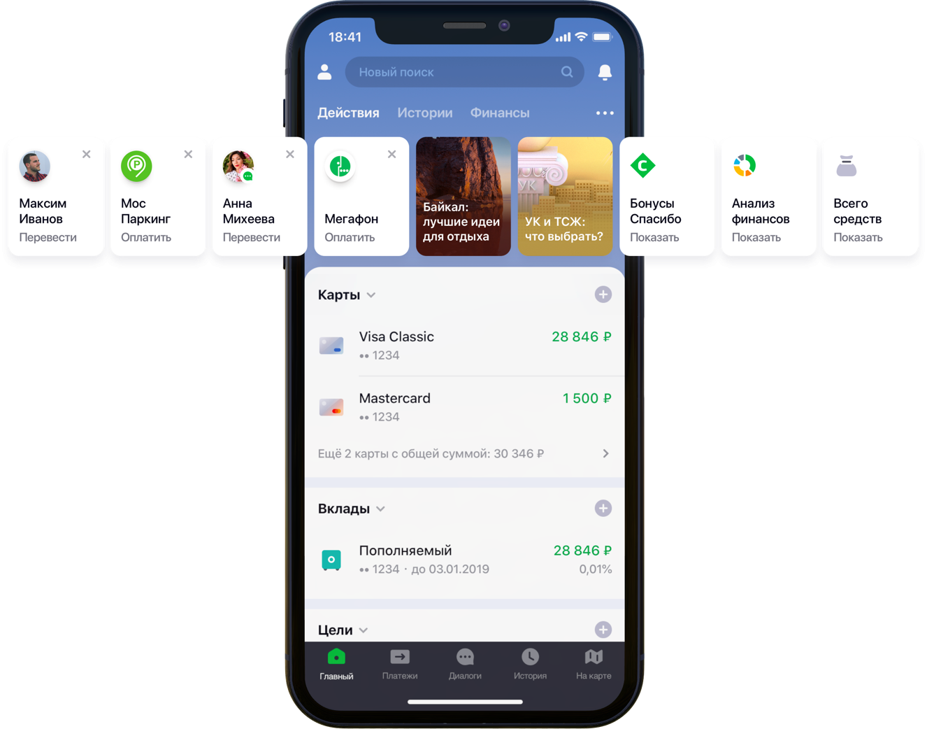
Design of the main screen of the mobile application with recommendations
We had 2 hundred thousand possible payment options, 55 million customers, 5 different banking sources, half a developer column and a mountain of banking activity, algorithms and all that, all colors, as well as a liter of random seeds, a box of hyperparameters, half a liter of correction factors and two dozens of libraries. Not that all this was necessary in the work, but since he began to improve the life of clients, then go in your hobby to the end. Under the cut is the story of the battle for UX, the correct formulation of the problem, the fight against the dimensionality of data, the contribution to open-source and our results.
')
As the development and scaling up, the Sberbank Online application is gaining useful features and additional functionality. In particular, in the application you can transfer money or pay for services of various organizations.
“We carefully looked at all the user paths inside the application and realized that many of them can be significantly reduced. To do this, we decided to personalize the main screen in several stages. First, we tried to remove from the screen what the client does not use, starting with bank cards. Then they brought to the fore those actions that the client had already performed before and for which he could go into the application right now. Now the list of actions includes payments to organizations and transfers to contacts, then the list of such actions will be expanded, ”said my colleague Sergey Komarov, who is developing the functionality from the point of view of the client in the Sberbank Online team. It is necessary to build a model that would fill the designated slots in the "Actions" widgets (figure above) with personal recommendations of payments and transfers instead of simple rules.
We in the team decomposed the task into two parts:
We decided to test the functionality first in the search tab:

Recommended Search Screen Design
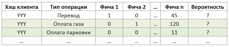
If we set the subtask as a recommendation to repeat operations, this allows us to get rid of the calculation and evaluation of trillions of combinations of all possible operations for all customers and focus on a much more limited number of them. If out of the whole set of operations available to our clients, the hypothetical client with the YYY hash used only gas and parking payments, then we will evaluate the probability of repeating only these operations for this client:
An example of reducing the dimension of data for scoring
The sample is a transactional observation, enriched with factors of client demography, financial aggregates and various frequency characteristics of a particular operation.
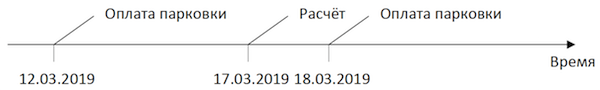
The target variable in this case is binary and reflects the fact of the event on the day following the day the factors are calculated. Thus, iteratively moving the day of calculating the factors and setting the flag of the target variable, we multiply and mark the same operations and mark them differently depending on the position relative to this day.
Observation Scheme
Calculating the slice on 03/17/2019 for the client “YYY”, we get two observations:

An example of the observations for a dataset
“Feature 1” can mean, for example, the balance on all cards of the client, “Feature 2” - the presence of this type of operation in the last week.
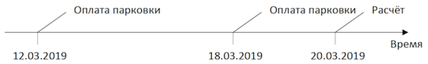
We take the same transactions, but form observations for training on a different date:
Observation Scheme
We get observations for a dataset with other values of both features and the target variable:

An example of the observations for a dataset
In the examples above, for clarity, the actual values of the factors are given, but in fact, the values are processed by an automatic algorithm: the results of the WOE conversion are fed to the input of the model. It allows you to bring the variables to a monotonic relationship with the target variable and at the same time get rid of the effects of outliers. For example, we have the factor “Number of cards” and some distribution of the target variable:

WOE conversion example
The WOE transformation allows us to transform a nonlinear dependence into at least a monotonic one. Each value of the analyzed factor is associated with its own WOE value and thus a new factor is formed, and the original one is removed from the dataset:

The effect of the WOE transform on the relationship with the target variable
The dictionary for converting variable values to WOE is saved and used later for scoring. That is, if we need to calculate the probabilities for tomorrow, we create a dataset as in the tables with examples of observations above, convert the necessary variables into WOE with the saved code, and apply the model on these data.
The choice of method was strictly limited - interpretability. Therefore, to comply with the deadlines, it was decided to postpone the explanations using the same SHAP in the second half of the problem and test relatively simple methods: regression and shallow neurons. The tool was SAS Miner, a software for preprocessing, analyzing, and building models on various data in an interactive form, which saves a lot of time on writing code.

SAS Miner Interface
Comparison of the GINI metric on an out-of-time sample showed that the neural network copes with the task best:
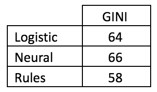
Comparative table of quality models and frequency rules
The model has two exit points. The recommendations in the form of widget cards on the main screen include operations whose forecast is above a certain threshold (see the first picture in the post). The border is selected based on a balance of quality and coverage, which in such an architecture is half of all operations performed. Top-4 operations are sent to the “recommended operations” block of the search screen (see the second picture).
Turning to the second part of the task, we return to the problem of a huge number of possible payment options for the services of providers that need to be evaluated and sorted within each client — trillions of pairs. In addition to this, we have implicit data, that is, there is no information about the assessment of payments made, or why the client did not make any payments. Therefore, to begin with, it was decided to test various methods of expanding the matrix of payments from customers to providers: ALS and FM.
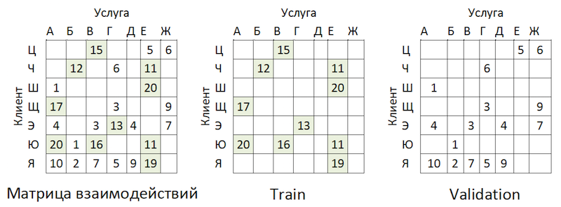
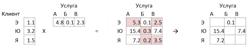
ALS (Alternating Least Squares) or Alternating Least Squares - in collaborative filtering, one of the methods for solving the problem of factorization of the interaction matrix. We will present our transactional data on payment of services in the form of a matrix in which columns are unique identifiers of all providers' services, and rows are unique customers. In the cells we place the number of operations of specific clients with specific providers for a certain period of time:

Matrix decomposition principle
The meaning of the method is that we create two such matrices of lower dimension, the multiplication of which gives the closest result to the original large matrix in the filled cells. The model learns to create a hidden factorial description for customers and for providers. An implementation of the method in the implicit library was used. Training takes place according to the following algorithm:
Transactional data was transformed into a matrix of interactions with a degree of sparseness of ~ 99% with great unevenness among providers. To separate the data into train and validation samples, we randomly masked the proportion of filled cells:
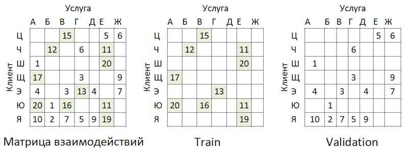
Data Sharing Example
Transactions were taken as a test for the time interval following the training, and laid out in a matrix of the same format - it turned out-of-time.
The model has several hyperparameters that can be adjusted to improve quality:
We used the hyperopt library, which allows us to evaluate the effect of hyperparameters on the quality metric using the TPE method and select their optimal value. The algorithm starts with a cold start and makes several estimates of the quality metric depending on the values of the analyzed hyperparameters. Then, in essence, he tries to select a set of hyperparameter values that is more likely to give a good value for the quality metric. The results are saved in a dictionary from which you can build a graph and visually evaluate the result of the optimizer (blue is better):
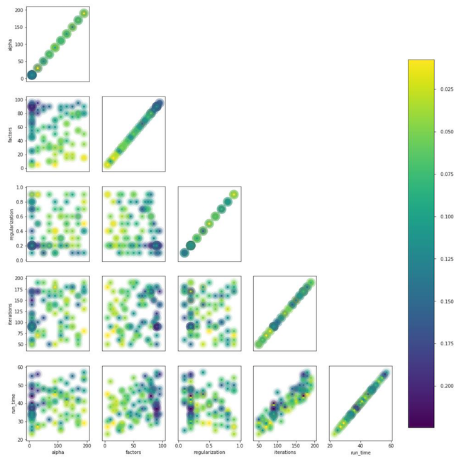
The graph of the dependence of the quality metric on the combination of hyperparameters
The graph shows that the values of the hyperparameters strongly affect the quality of the model. Since it is necessary to apply ranges for each of them to the input of the method, the graph can further determine whether it makes sense to expand the value space or not. For example, in our task it is clear that it makes sense to test large values for the number of factors. In the future, this really improved the model.
How to evaluate the quality of the model? One of the most commonly used metrics for recommender systems where order is important is MAP @ k or Mean Average Precision at K. This metric estimates the accuracy of the model on K recommendations taking into account the order of the items in the list of these recommendations on average for all clients.
Unfortunately, a quality assessment operation even on a sample took several hours. Having rolled up our sleeves, we started profiling the mean_average_pecision_at_k () function with the line_profiler library. The task was further complicated by the fact that the function used cython code and had to be correctly taken into account , otherwise the necessary statistics were simply not collected. As a result, we again faced the problem of the dimensionality of our data. To calculate this metric, you need to get some estimates of each service from all possible for each client and select the top-K personal recommendations by sorting from the resulting array. Even considering the use of partial sorting of numpy.argpartition () with O (n) complexity, sorting the grades turned out to be the longest step, stretching the quality score to the clock. Since numpy.argpartition () did not use all the kernels of our server, it was decided to improve the algorithm by rewriting this part in C ++ and OpenMP via cython. A briefly new algorithm is as follows:
This allowed us to speed up the calculation of recommendations several times. The revision has been added to the official repository.
And now it's time to evaluate the quality of the model. Why do we need out-of-time sampling? If we look at the distribution of operations by providers, we will see the following picture:
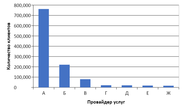
Distribution of popularity of service providers
There is an imbalance. This leads to the fact that the model is trying to recommend popular services. Back to the picture above:
The problem is that if you check the accuracy of the model by masking the same matrix, as is advised almost everywhere, then for most clients (marginal examples: “W”, “E” and “I”) the quality of the validation forecasts (we will pretend that she did not participate in the selection of hyperparameters) will be high if these are the most popular providers. As a result, we get a false confidence in the strength of the model. Therefore, we acted as follows:
The logic of preparing the matrix for generating forecasts
As a base line, we compiled a list of providers, sorted by popularity, and multiplied it by all customers, again excluding the existing client-service pairs. It turned out to be sad and not at all what we expected and saw on the train \ validation samples:

Comparison chart of model quality and baseline
Stop! We have client factors and parameters of providers. We get factorization machines.
Factorization machines (factorization machine) - a learning algorithm with a teacher, designed to find relationships between factors that describe interacting entities, which are presented in the form of sparse matrices. We used the implementation of FM from the LightFM library.
In addition to the normalized interaction matrix, the method uses two additional datasets with factors for customers and for the services of providers in the form of one-hot-encoded matrices connected to single ones:
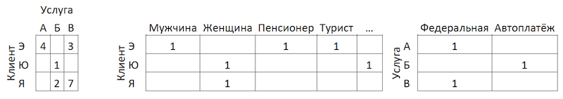
The logic of preparing the matrix for generating forecasts
The quality of the FM model on our data turned out to be lower than ALS:

Comparative table of quality models and baseline
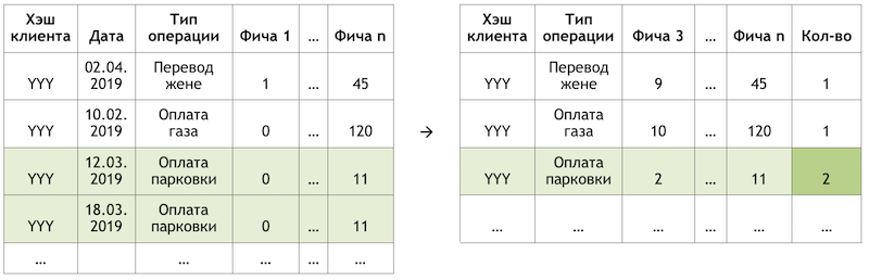
It was decided to come in from the other side. Remembering the distribution of the popularity of services, we identified 300 of them, transactions for which cover 80% of all operations, and trained a classifier on them. Here, the data represents aggregates of customer transactions enriched with client features:
Transaction aggregation scheme
Why only client-side, you ask? Because in this case, to prepare recommendations, it will be enough for us to have one line per client. Applying the model to it, we get the output vector of probabilities for all classes, from which it is easy to choose top-K recommendations. If we add the features of provider services to the training set, then at the stage of applying the model we will have to either prepare 300 lines for each client - one for each provider service with features that describe them, or build another model for pre-sorting scoring candidates .
Adding features to clients from ALS did not increase our data, since we already took into account transactional activity - for example, in sections of the MCC or categories in the style of "gamer" or "theater". In this format, we managed to get good results:
Comparative table of quality models and baseline
Despite the high quality of the model, one more problem remains in this approach. Since the architecture of the data and model does not imply the use of features of the services of providers, the model does not fully take into account geography and may recommend that people pay for the service of a local provider from another region. To minimize this risk, we have developed a small filter to pre-cut options before entering recommendations. An easy fleur of recursion is thrown on the algorithm:
After these manipulations using the Herfindahl index, we separate the regional providers, which are represented in a limited set of regions, from the federal ones:

Separation of providers by presence in the regions
We form a mask with acceptable regional providers for customers and exclude unnecessary items from model predictions before creating a list of recommendations.
We have developed two models that together form a complete set of recommendations on payments and transfers. It was possible to reduce the client path for half the recurring operations to one click. In future plans to improve the model of “recommended operations” using feedback data (cards can be hidden, etc.), which will reduce the threshold for selecting recommendations and increase coverage. It is also planned to expand the coverage of recommended payments in the model of “search examples” and develop an algorithm for scoring optimization for it.
We have gone through the thorny path of building a recommender system of payments and transfers. On the way, we got bumps and gained experience in decomposing and simplifying such tasks, correctly evaluating such systems, applicability of methods, optimal work with large amounts of data, and significantly expanded our understanding of the specifics of such tasks. Along the way, I managed to contribute to the open-source, which we ourselves use. I wish you interesting tasks, realistic baselines and single F1. Thanks for attention!
Design of the main screen of the mobile application with recommendations
We had 2 hundred thousand possible payment options, 55 million customers, 5 different banking sources, half a developer column and a mountain of banking activity, algorithms and all that, all colors, as well as a liter of random seeds, a box of hyperparameters, half a liter of correction factors and two dozens of libraries. Not that all this was necessary in the work, but since he began to improve the life of clients, then go in your hobby to the end. Under the cut is the story of the battle for UX, the correct formulation of the problem, the fight against the dimensionality of data, the contribution to open-source and our results.
')
Formulation of the problem
As the development and scaling up, the Sberbank Online application is gaining useful features and additional functionality. In particular, in the application you can transfer money or pay for services of various organizations.
“We carefully looked at all the user paths inside the application and realized that many of them can be significantly reduced. To do this, we decided to personalize the main screen in several stages. First, we tried to remove from the screen what the client does not use, starting with bank cards. Then they brought to the fore those actions that the client had already performed before and for which he could go into the application right now. Now the list of actions includes payments to organizations and transfers to contacts, then the list of such actions will be expanded, ”said my colleague Sergey Komarov, who is developing the functionality from the point of view of the client in the Sberbank Online team. It is necessary to build a model that would fill the designated slots in the "Actions" widgets (figure above) with personal recommendations of payments and transfers instead of simple rules.
Decision
We in the team decomposed the task into two parts:
- the recommendation of the repetition of operations to pay for services or transfer funds (block “Recommended operations”)
- recommendation of examples of search requests for payment for services not previously used by this client (block “Search Examples”)
We decided to test the functionality first in the search tab:
Recommended Search Screen Design
Recommended Operations
Scoring optimization
If we set the subtask as a recommendation to repeat operations, this allows us to get rid of the calculation and evaluation of trillions of combinations of all possible operations for all customers and focus on a much more limited number of them. If out of the whole set of operations available to our clients, the hypothetical client with the YYY hash used only gas and parking payments, then we will evaluate the probability of repeating only these operations for this client:
An example of reducing the dimension of data for scoring
Preparing the dataset
The sample is a transactional observation, enriched with factors of client demography, financial aggregates and various frequency characteristics of a particular operation.
The target variable in this case is binary and reflects the fact of the event on the day following the day the factors are calculated. Thus, iteratively moving the day of calculating the factors and setting the flag of the target variable, we multiply and mark the same operations and mark them differently depending on the position relative to this day.
Observation Scheme
Calculating the slice on 03/17/2019 for the client “YYY”, we get two observations:
An example of the observations for a dataset
“Feature 1” can mean, for example, the balance on all cards of the client, “Feature 2” - the presence of this type of operation in the last week.
We take the same transactions, but form observations for training on a different date:
Observation Scheme
We get observations for a dataset with other values of both features and the target variable:
An example of the observations for a dataset
In the examples above, for clarity, the actual values of the factors are given, but in fact, the values are processed by an automatic algorithm: the results of the WOE conversion are fed to the input of the model. It allows you to bring the variables to a monotonic relationship with the target variable and at the same time get rid of the effects of outliers. For example, we have the factor “Number of cards” and some distribution of the target variable:
WOE conversion example
The WOE transformation allows us to transform a nonlinear dependence into at least a monotonic one. Each value of the analyzed factor is associated with its own WOE value and thus a new factor is formed, and the original one is removed from the dataset:
The effect of the WOE transform on the relationship with the target variable
The dictionary for converting variable values to WOE is saved and used later for scoring. That is, if we need to calculate the probabilities for tomorrow, we create a dataset as in the tables with examples of observations above, convert the necessary variables into WOE with the saved code, and apply the model on these data.
Training
The choice of method was strictly limited - interpretability. Therefore, to comply with the deadlines, it was decided to postpone the explanations using the same SHAP in the second half of the problem and test relatively simple methods: regression and shallow neurons. The tool was SAS Miner, a software for preprocessing, analyzing, and building models on various data in an interactive form, which saves a lot of time on writing code.
SAS Miner Interface
Quality control
Comparison of the GINI metric on an out-of-time sample showed that the neural network copes with the task best:
Comparative table of quality models and frequency rules
The model has two exit points. The recommendations in the form of widget cards on the main screen include operations whose forecast is above a certain threshold (see the first picture in the post). The border is selected based on a balance of quality and coverage, which in such an architecture is half of all operations performed. Top-4 operations are sent to the “recommended operations” block of the search screen (see the second picture).
Search Examples
Turning to the second part of the task, we return to the problem of a huge number of possible payment options for the services of providers that need to be evaluated and sorted within each client — trillions of pairs. In addition to this, we have implicit data, that is, there is no information about the assessment of payments made, or why the client did not make any payments. Therefore, to begin with, it was decided to test various methods of expanding the matrix of payments from customers to providers: ALS and FM.
ALS
ALS (Alternating Least Squares) or Alternating Least Squares - in collaborative filtering, one of the methods for solving the problem of factorization of the interaction matrix. We will present our transactional data on payment of services in the form of a matrix in which columns are unique identifiers of all providers' services, and rows are unique customers. In the cells we place the number of operations of specific clients with specific providers for a certain period of time:
Matrix decomposition principle
The meaning of the method is that we create two such matrices of lower dimension, the multiplication of which gives the closest result to the original large matrix in the filled cells. The model learns to create a hidden factorial description for customers and for providers. An implementation of the method in the implicit library was used. Training takes place according to the following algorithm:
- The matrix of clients and providers with hidden factors is initialized. Their number is the hyperparameter of the model.
- The matrix of hidden factors of providers is fixed and the derivative of the loss function for the correction of the client matrix is considered. The author used an interesting method of conjugate gradients , which allows you to greatly accelerate this step.
- The previous step is repeated similarly for the matrix of hidden factors of customers.
- Steps 2-3 alternate until the algorithm converges.
Training
Transactional data was transformed into a matrix of interactions with a degree of sparseness of ~ 99% with great unevenness among providers. To separate the data into train and validation samples, we randomly masked the proportion of filled cells:
Data Sharing Example
Transactions were taken as a test for the time interval following the training, and laid out in a matrix of the same format - it turned out-of-time.
Training
The model has several hyperparameters that can be adjusted to improve quality:
- Alpha is the coefficient by which the matrix is weighted, adjusting the degree of confidence ( C_iu ) that the given service of the provider really “likes” the client.
- The number of factors in the hidden matrices of clients and providers is the number of columns and rows, respectively.
- Regularization coefficient L2 λ.
- The number of iterations of the method.
We used the hyperopt library, which allows us to evaluate the effect of hyperparameters on the quality metric using the TPE method and select their optimal value. The algorithm starts with a cold start and makes several estimates of the quality metric depending on the values of the analyzed hyperparameters. Then, in essence, he tries to select a set of hyperparameter values that is more likely to give a good value for the quality metric. The results are saved in a dictionary from which you can build a graph and visually evaluate the result of the optimizer (blue is better):
The graph of the dependence of the quality metric on the combination of hyperparameters
The graph shows that the values of the hyperparameters strongly affect the quality of the model. Since it is necessary to apply ranges for each of them to the input of the method, the graph can further determine whether it makes sense to expand the value space or not. For example, in our task it is clear that it makes sense to test large values for the number of factors. In the future, this really improved the model.
Quality assessment metric and complexity
How to evaluate the quality of the model? One of the most commonly used metrics for recommender systems where order is important is MAP @ k or Mean Average Precision at K. This metric estimates the accuracy of the model on K recommendations taking into account the order of the items in the list of these recommendations on average for all clients.
Unfortunately, a quality assessment operation even on a sample took several hours. Having rolled up our sleeves, we started profiling the mean_average_pecision_at_k () function with the line_profiler library. The task was further complicated by the fact that the function used cython code and had to be correctly taken into account , otherwise the necessary statistics were simply not collected. As a result, we again faced the problem of the dimensionality of our data. To calculate this metric, you need to get some estimates of each service from all possible for each client and select the top-K personal recommendations by sorting from the resulting array. Even considering the use of partial sorting of numpy.argpartition () with O (n) complexity, sorting the grades turned out to be the longest step, stretching the quality score to the clock. Since numpy.argpartition () did not use all the kernels of our server, it was decided to improve the algorithm by rewriting this part in C ++ and OpenMP via cython. A briefly new algorithm is as follows:
- Data is cut into batches by customers.
- An empty matrix and pointers to memory are initialized.
- Batches strings by pointers are sorted in two ways: by the partial_sort function and then sort by the C ++ algorithm library.
- The results are written to the cells of the empty matrix in parallel.
- Data is returned in python.
This allowed us to speed up the calculation of recommendations several times. The revision has been added to the official repository.
OOT Results Analysis
And now it's time to evaluate the quality of the model. Why do we need out-of-time sampling? If we look at the distribution of operations by providers, we will see the following picture:
Distribution of popularity of service providers
There is an imbalance. This leads to the fact that the model is trying to recommend popular services. Back to the picture above:
The problem is that if you check the accuracy of the model by masking the same matrix, as is advised almost everywhere, then for most clients (marginal examples: “W”, “E” and “I”) the quality of the validation forecasts (we will pretend that she did not participate in the selection of hyperparameters) will be high if these are the most popular providers. As a result, we get a false confidence in the strength of the model. Therefore, we acted as follows:
- Formed estimates of providers by model.
- The existing client-service pairs were excluded from the ratings (see the figure below) and OOT-matrices.
- Formed from the remaining ratings of the top-K recommendations and rated MAP @ k on the remaining OOT.
The logic of preparing the matrix for generating forecasts
As a base line, we compiled a list of providers, sorted by popularity, and multiplied it by all customers, again excluding the existing client-service pairs. It turned out to be sad and not at all what we expected and saw on the train \ validation samples:
Comparison chart of model quality and baseline
Stop! We have client factors and parameters of providers. We get factorization machines.
FM
Factorization machines (factorization machine) - a learning algorithm with a teacher, designed to find relationships between factors that describe interacting entities, which are presented in the form of sparse matrices. We used the implementation of FM from the LightFM library.
Data format
In addition to the normalized interaction matrix, the method uses two additional datasets with factors for customers and for the services of providers in the form of one-hot-encoded matrices connected to single ones:
The logic of preparing the matrix for generating forecasts
Quality control
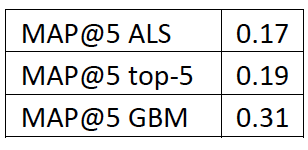
The quality of the FM model on our data turned out to be lower than ALS:
Comparative table of quality models and baseline
Change Model Architecture - Boosting
It was decided to come in from the other side. Remembering the distribution of the popularity of services, we identified 300 of them, transactions for which cover 80% of all operations, and trained a classifier on them. Here, the data represents aggregates of customer transactions enriched with client features:
Transaction aggregation scheme
Why only client-side, you ask? Because in this case, to prepare recommendations, it will be enough for us to have one line per client. Applying the model to it, we get the output vector of probabilities for all classes, from which it is easy to choose top-K recommendations. If we add the features of provider services to the training set, then at the stage of applying the model we will have to either prepare 300 lines for each client - one for each provider service with features that describe them, or build another model for pre-sorting scoring candidates .
Adding features to clients from ALS did not increase our data, since we already took into account transactional activity - for example, in sections of the MCC or categories in the style of "gamer" or "theater". In this format, we managed to get good results:
Comparative table of quality models and baseline
Regional filter
Despite the high quality of the model, one more problem remains in this approach. Since the architecture of the data and model does not imply the use of features of the services of providers, the model does not fully take into account geography and may recommend that people pay for the service of a local provider from another region. To minimize this risk, we have developed a small filter to pre-cut options before entering recommendations. An easy fleur of recursion is thrown on the algorithm:
- We collect information about the client’s region from bank profiles and other internal sources.
- We select the main regions of presence for each provider.
- We clarify / fill in the information about the client’s region by the regions of the providers that he uses.
After these manipulations using the Herfindahl index, we separate the regional providers, which are represented in a limited set of regions, from the federal ones:
Separation of providers by presence in the regions
We form a mask with acceptable regional providers for customers and exclude unnecessary items from model predictions before creating a list of recommendations.
Conclusion
We have developed two models that together form a complete set of recommendations on payments and transfers. It was possible to reduce the client path for half the recurring operations to one click. In future plans to improve the model of “recommended operations” using feedback data (cards can be hidden, etc.), which will reduce the threshold for selecting recommendations and increase coverage. It is also planned to expand the coverage of recommended payments in the model of “search examples” and develop an algorithm for scoring optimization for it.
We have gone through the thorny path of building a recommender system of payments and transfers. On the way, we got bumps and gained experience in decomposing and simplifying such tasks, correctly evaluating such systems, applicability of methods, optimal work with large amounts of data, and significantly expanded our understanding of the specifics of such tasks. Along the way, I managed to contribute to the open-source, which we ourselves use. I wish you interesting tasks, realistic baselines and single F1. Thanks for attention!
Source: https://habr.com/ru/post/461747/
All Articles