The collection, storage, transformation and presentation of data are the main challenges facing data engineers. The Business Intelligence Badoo department receives and processes more than 20 billion events sent from user devices per day, or 2 TB of incoming data.

The study and interpretation of all this data is not always a trivial task, sometimes there is a need to go beyond the capabilities of ready-made databases. And if you have the courage and decided to do something new, you should first familiarize yourself with the working principles of existing solutions.

In a word, curious and strong-minded developers, this article is addressed. In it you will find a description of the traditional model of query execution in relational databases using the demo language PigletQL as an example.

Content

• Background
• SQL interpreter structure
• Volcano Model and Query Execution
• PigletQL
  
  • Lexical and parser
  • Semantic analyzer
  • Compiling Queries into an Intermediate View
  • Execution of the intermediate representation
  • Operators
  • Work examples
• findings
• Literature

Background

Our group of engineers is engaged in backends and interfaces, providing opportunities for analysis and research of data within the company (by the way, we are expanding ). Our standard tools are a distributed database of dozens of servers (Exasol) and a Hadoop cluster for hundreds of machines (Hive and Presto).

Most of the queries to these databases are analytical, that is, affecting from hundreds of thousands to billions of records. Their execution takes minutes, tens of minutes or even hours, depending on the solution used and the complexity of the request. With manual work of the user-analyst, such time is considered acceptable, but is not suitable for interactive research through the user interface.

Over time, we highlighted the popular analytical queries and queries, which are difficult to set out in terms of SQL, and developed small specialized databases for them. They store a subset of data in a format suitable for lightweight compression algorithms (for example, streamvbyte), which allows you to store data in a single machine for several days and execute queries in seconds.

The first query languages ​​for these data and their interpreters were implemented on a hunch, we had to constantly refine them, and each time it took an unacceptably long time.

Query languages ​​were not flexible enough, although there were no obvious reasons for limiting their capabilities. As a result, we turned to the experience of developers of SQL interpreters, thanks to which we were able to partially solve the problems that arose.

Below I will talk about the most common query execution model in relational databases - Volcano. The source code of the interpreter of the primitive SQL dialect, PigletQL , is attached to the article , so everyone who is interested can easily get acquainted with the details in the repository.

SQL interpreter structure

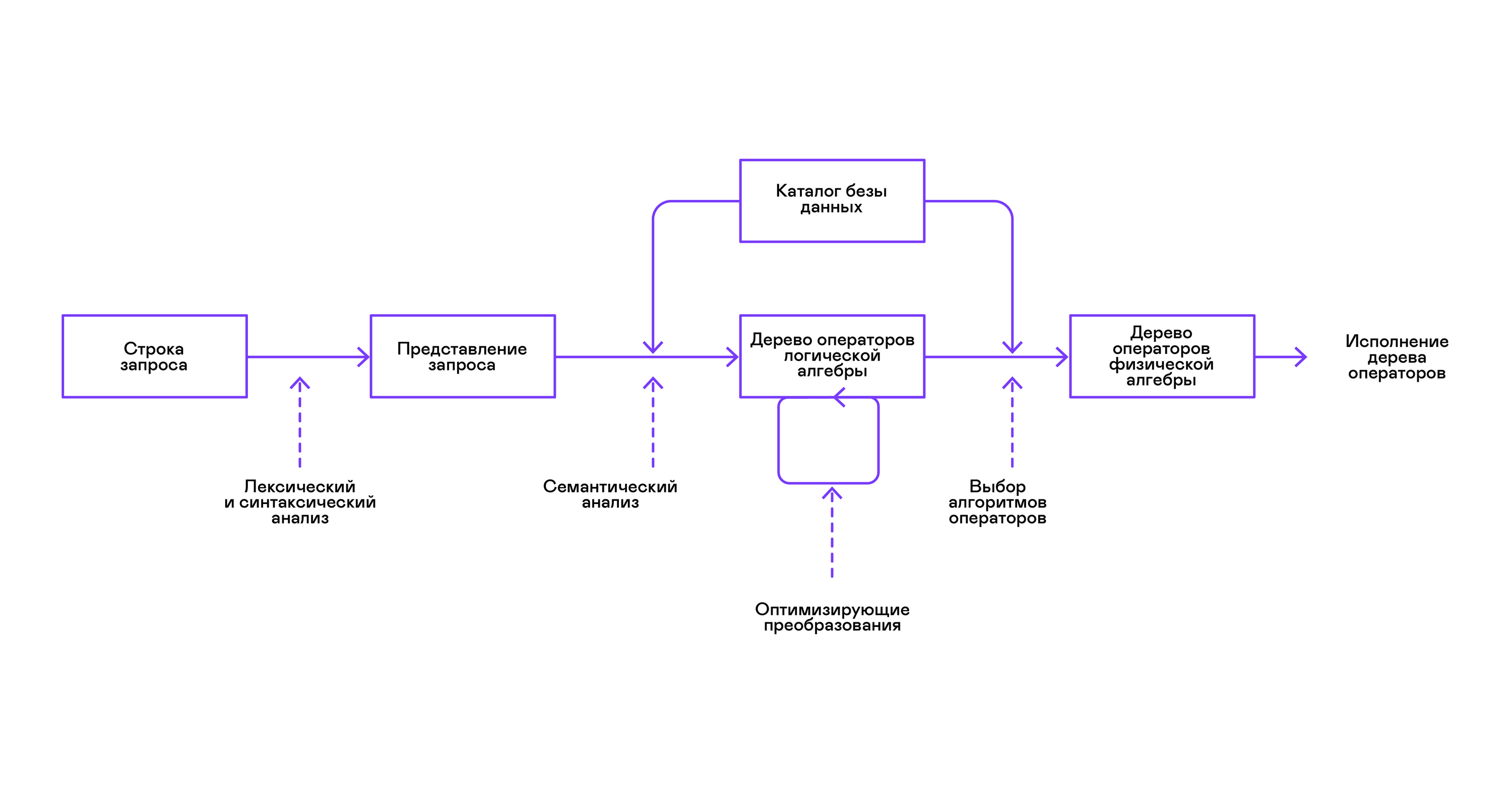
Most popular databases provide an interface to data in the form of a declarative SQL query language. A query in the form of a string is converted by the parser into a query description similar to an abstract syntax tree. It is possible to execute simple queries already at this stage, however, for optimizing transformations and subsequent execution, this representation is inconvenient. In the databases known to me, intermediate representations are introduced for these purposes.

Relational algebra became a model for intermediate representations. This is a language where the transformations ( operators ) performed on the data are explicitly described: selecting a subset of data according to a predicate, combining data from different sources, etc. In addition, relational algebra is an algebra in the mathematical sense, that is, a large number of equivalent transformations. Therefore, it is convenient to carry out optimizing transformations over a query in the form of a tree of relational algebra operators.

There are important differences between internal representations in databases and the original relational algebra, so it’s more correct to call it logical algebra .

The validation of a query is usually performed when compiling the initial representation of the query into logical algebra operators and corresponds to the stage of semantic analysis in conventional compilers. The role of the symbol table in databases is played by the database directory , which stores information about the database schema and metadata: tables, table columns, indexes, user rights, etc.

Compared with general-purpose interpreters, database interpreters have one more peculiarity: differences in the volume of data and meta-information about the data to which queries are supposed to be made. In tables, or relations in terms of relational algebra, there can be a different amount of data, on some columns (relationship attributes ) indexes can be built, etc. That is, depending on the database schema and the amount of data in the tables, the query must be performed by different algorithms , and use them in a different order.

To solve this problem, another intermediate representation is introduced - physical algebra . Depending on the availability of indexes on the columns, the amount of data in the tables, and the structure of the tree of logical algebra, different forms of the tree of physical algebra are offered, from which the best option is chosen. It is this tree that is shown to the database as a query plan. In conventional compilers, this stage conditionally corresponds to the stages of register allocation, planning, and instruction selection.

The last step in the work of the interpreter is directly the execution of the tree of operators of physical algebra.

Volcano Model and Query Execution

Physical algebra tree interpreters have always been used in closed commercial databases, but academic literature usually refers to the experimental optimizer Volcano, developed in the early 90's.

In the Volcano model, each operator of a tree of physical algebra turns into a structure with three functions: open, next, close. In addition to functions, the operator contains an operating state - state. The open function initiates the state of the statement, the next function returns either the next tuple (English tuple), or NULL, if there are no tuples left, the close function terminates the statement:

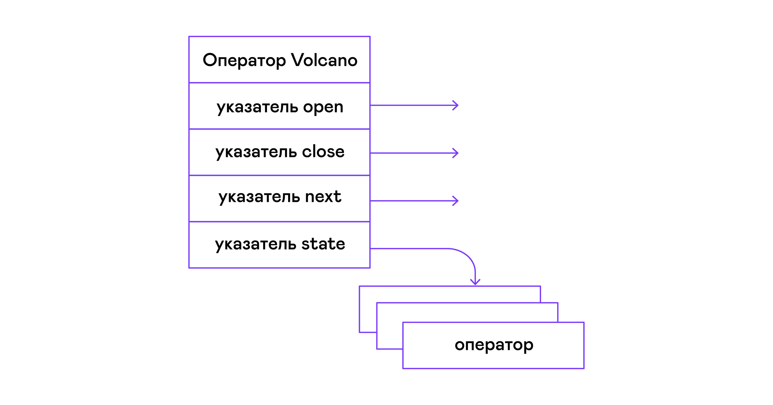
Operators can be nested to form a tree of operators of physical algebra. Each operator, thus, iterates over the tuples of either a relation existing on a real medium or a virtual relation formed by enumerating the tuples of nested operators:

In terms of modern high-level languages, the tree of such operators is a cascade of iterators.

Even industrial query interpreters in relational DBMS are repelled from the Volcano model, so I took it as the basis for the PigletQL interpreter.

PigletQL

To demonstrate the model, I developed the interpreter of the limited query language PigletQL . It is written in C, supports the creation of tables in the style of SQL, but is limited to a single type - 32-bit positive integers. All tables are in memory. The system operates in a single thread and does not have a transaction mechanism.

There is no optimizer in PigletQL and SELECT queries are compiled directly into the operator tree of physical algebra. The remaining queries (CREATE TABLE and INSERT) work directly from the primary internal views.

Example user session in PigletQL:

> ./pigletql > CREATE TABLE tab1 (col1,col2,col3); > INSERT INTO tab1 VALUES (1,2,3); > INSERT INTO tab1 VALUES (4,5,6); > SELECT col1,col2,col3 FROM tab1; col1 col2 col3 1 2 3 4 5 6 rows: 2 > SELECT col1 FROM tab1 ORDER BY col1 DESC; col1 4 1 rows: 2 

Lexical and parser

PigletQL is a very simple language, and its implementation was not required at the stages of lexical and parsing analysis.

The lexical analyzer is written by hand. An analyzer object ( scanner_t ) is created from the query string, which returns tokens one by one:

 scanner_t *scanner_create(const char *string); void scanner_destroy(scanner_t *scanner); token_t scanner_next(scanner_t *scanner); 

Parsing is done using the recursive descent method. First, the parser_t object is created , which, having received the lexical analyzer (scanner_t), fills the query_t object with information about the request:

 query_t *query_create(void); void query_destroy(query_t *query); parser_t *parser_create(void); void parser_destroy(parser_t *parser); bool parser_parse(parser_t *parser, scanner_t *scanner, query_t *query); 

The result of parsing in query_t is one of the three types of query supported by PigletQL:

 typedef enum query_tag { QUERY_SELECT, QUERY_CREATE_TABLE, QUERY_INSERT, } query_tag; /* * ... query_select_t, query_create_table_t, query_insert_t definitions ... **/ typedef struct query_t { query_tag tag; union { query_select_t select; query_create_table_t create_table; query_insert_t insert; } as; } query_t; 

The most complex kind of query in PigletQL is SELECT. It corresponds to the query_select_t data structure :

 typedef struct query_select_t { /* Attributes to output */ attr_name_t attr_names[MAX_ATTR_NUM]; uint16_t attr_num; /* Relations to get tuples from */ rel_name_t rel_names[MAX_REL_NUM]; uint16_t rel_num; /* Predicates to apply to tuples */ query_predicate_t predicates[MAX_PRED_NUM]; uint16_t pred_num; /* Pick an attribute to sort by */ bool has_order; attr_name_t order_by_attr; sort_order_t order_type; } query_select_t; 

The structure contains a description of the query (an array of attributes requested by the user), a list of data sources - relationships, an array of predicates filtering tuples, and information about the attribute used to sort the results.

Semantic analyzer

The semantic analysis phase in regular SQL involves checking for the existence of the listed tables, columns in the tables, and type checking in query expressions. For checks related to tables and columns, the database directory is used, where all information about the data structure is stored.

There are no complex expressions in PigletQL, so query checking is reduced to checking catalog metadata of tables and columns. SELECT queries, for example, are validated by the validate_select function. I will bring it in abbreviated form:

 static bool validate_select(catalogue_t *cat, const query_select_t *query) { /* All the relations should exist */ for (size_t rel_i = 0; rel_i < query->rel_num; rel_i++) { if (catalogue_get_relation(cat, query->rel_names[rel_i])) continue; fprintf(stderr, "Error: relation '%s' does not exist\n", query->rel_names[rel_i]); return false; } /* Relation names should be unique */ if (!rel_names_unique(query->rel_names, query->rel_num)) return false; /* Attribute names should be unique */ if (!attr_names_unique(query->attr_names, query->attr_num)) return false; /* Attributes should be present in relations listed */ /* ... */ /* ORDER BY attribute should be available in the list of attributes chosen */ /* ... */ /* Predicate attributes should be available in the list of attributes projected */ /* ... */ return true; } 

If the request is valid, then the next step is to compile the parse tree into an operator tree.

Compiling Queries into an Intermediate View

In full-fledged SQL interpreters, there are usually two intermediate representations: logical and physical algebra.

A simple PigletQL interpreter performs CREATE TABLE and INSERT queries directly from its parsing trees, i.e. query_create_table_t and query_insert_t structures . More complex SELECT queries are compiled into a single intermediate representation, which will be executed by the interpreter.

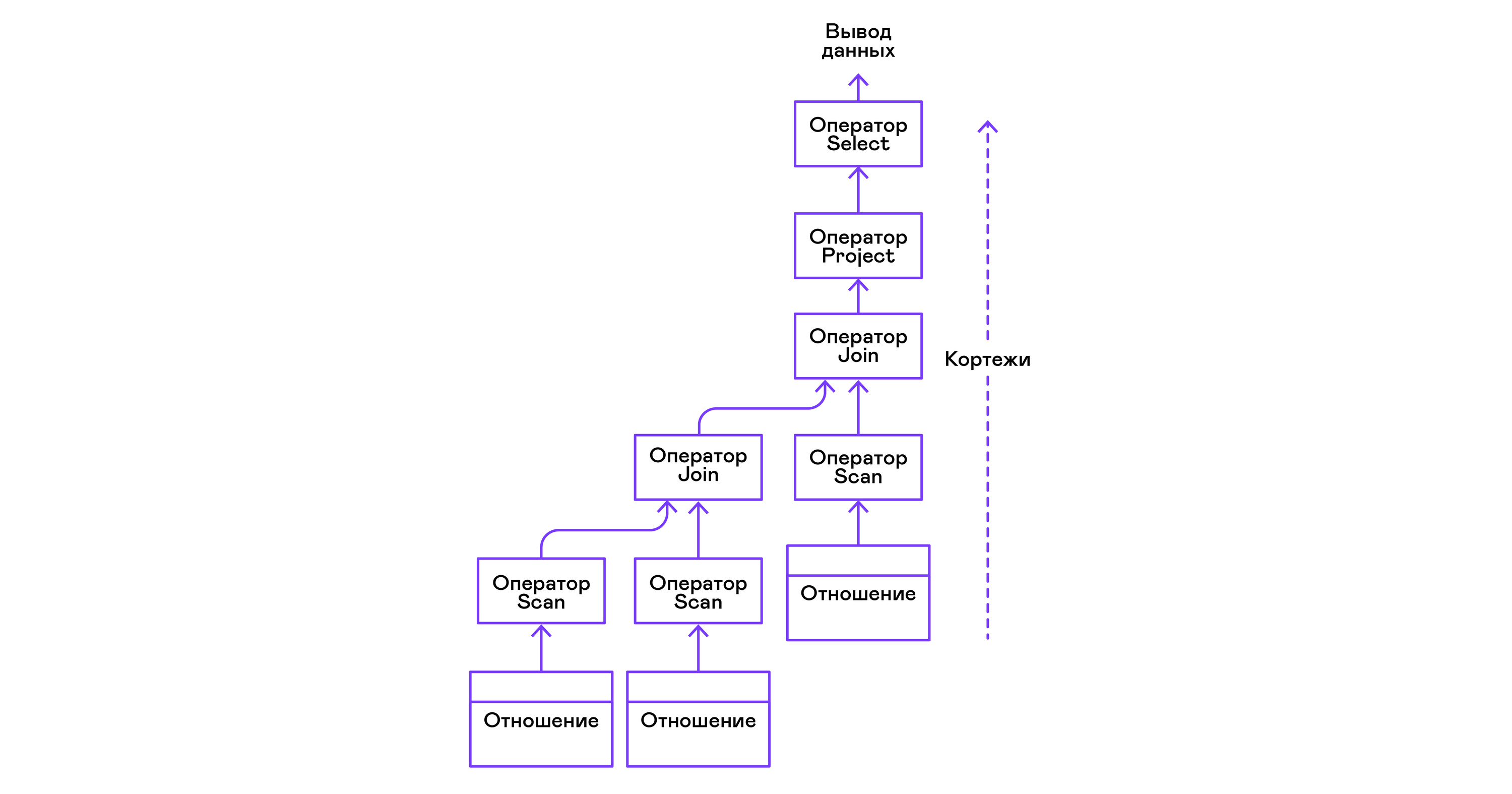
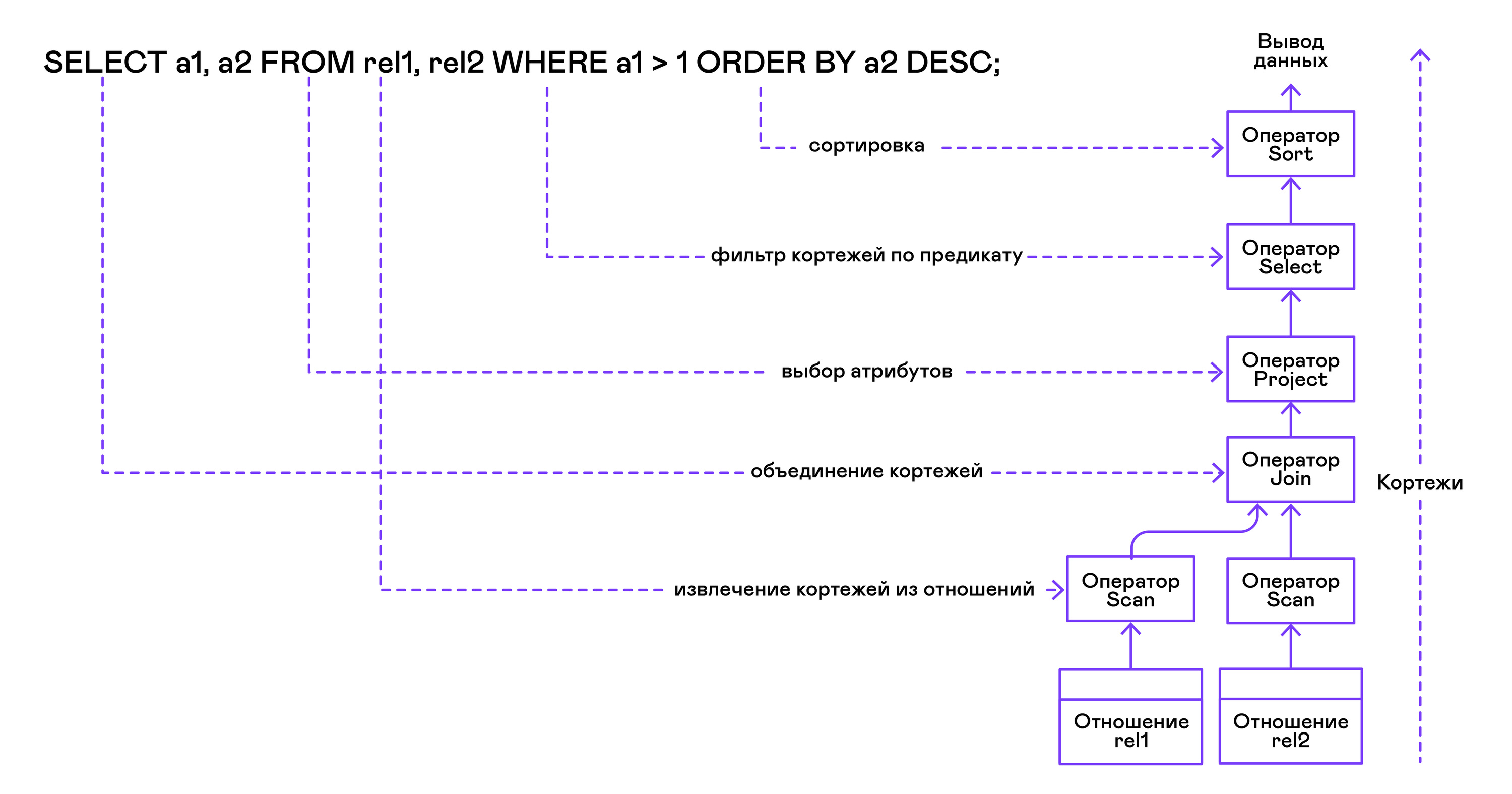
The operator tree is built from leaves to root in the following sequence:

1. From the right part of the query ("... FROM relation1, relation2, ..."), the names of the desired relations are obtained, for each of which a scan statement is created.

   
   

2. Extracting tuples from relations, scan operators are combined into a left-sided binary tree through the join operator.

   
   

3. Attributes requested by the user ("SELECT attr1, attr2, ...") are selected by the project statement.

   
   

4. If any predicates are specified ("... WHERE a = 1 AND b> 10 ..."), then the select statement is added to the tree above.

   
   

5. If the method for sorting the result is specified ("... ORDER BY attr1 DESC"), then the sort operator is added to the top of the tree.

   
   

Compilation in PigletQL code :

 operator_t *compile_select(catalogue_t *cat, const query_select_t *query) { /* Current root operator */ operator_t *root_op = NULL; /* 1. Scan ops */ /* 2. Join ops*/ { size_t rel_i = 0; relation_t *rel = catalogue_get_relation(cat, query->rel_names[rel_i]); root_op = scan_op_create(rel); rel_i += 1; for (; rel_i < query->rel_num; rel_i++) { rel = catalogue_get_relation(cat, query->rel_names[rel_i]); operator_t *scan_op = scan_op_create(rel); root_op = join_op_create(root_op, scan_op); } } /* 3. Project */ root_op = proj_op_create(root_op, query->attr_names, query->attr_num); /* 4. Select */ if (query->pred_num > 0) { operator_t *select_op = select_op_create(root_op); for (size_t pred_i = 0; pred_i < query->pred_num; pred_i++) { query_predicate_t predicate = query->predicates[pred_i]; /* Add a predicate to the select operator */ /* ... */ } root_op = select_op; } /* 5. Sort */ if (query->has_order) root_op = sort_op_create(root_op, query->order_by_attr, query->order_type); return root_op; } 

After the tree is formed, optimization transformations are usually carried out, but PigletQL immediately proceeds to the stage of execution of the intermediate representation.

Execution of the intermediate representation

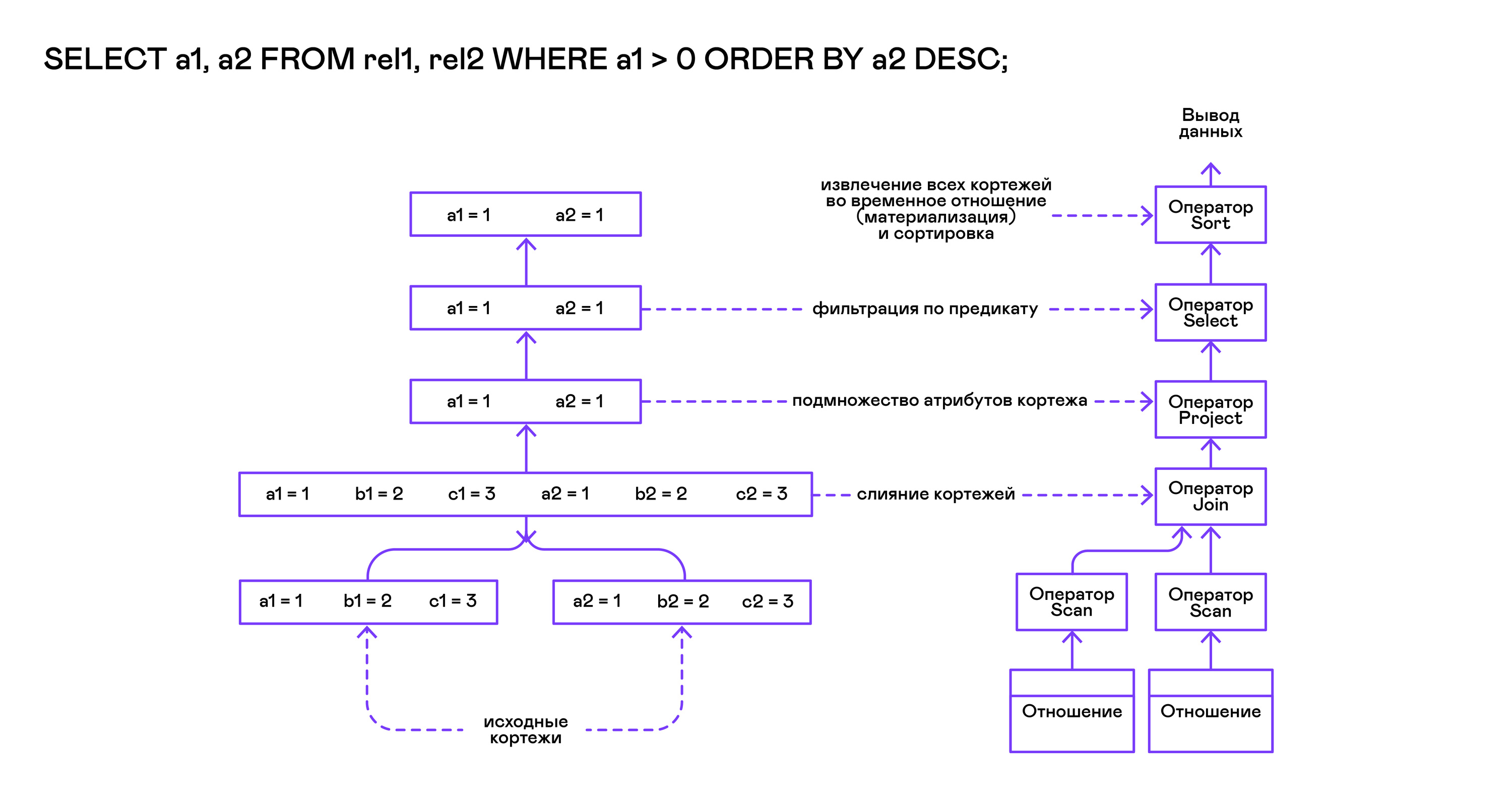
The Volcano model implies an interface for working with operators through three common open / next / close operations. In essence, each Volcano statement is an iterator from which tuples are “pulled” one by one, therefore this approach to execution is also called a pull model.

Each of these iterators can itself call the same functions of nested iterators, create temporary tables with intermediate results, and convert incoming tuples.

Executing SELECT queries in PigletQL:

 bool eval_select(catalogue_t *cat, const query_select_t *query) { /* Compile the operator tree: */ operator_t *root_op = compile_select(cat, query); /* Eval the tree: */ { root_op->open(root_op->state); size_t tuples_received = 0; tuple_t *tuple = NULL; while((tuple = root_op->next(root_op->state))) { /* attribute list for the first row only */ if (tuples_received == 0) dump_tuple_header(tuple); /* A table of tuples */ dump_tuple(tuple); tuples_received++; } printf("rows: %zu\n", tuples_received); root_op->close(root_op->state); } root_op->destroy(root_op); return true; } 

The request is first compiled by the compile_select function, which returns the root of the operator tree, after which the same open / next / close functions are called on the root operator. Each call to next returns either the next tuple or NULL. In the latter case, this means that all tuples have been extracted, and the close iterator function should be called.

The resulting tuples are recalculated and output by the table to the standard output stream.

Operators

The most interesting thing about PigletQL is the operator tree. I will show the device of some of them.

The operators have a common interface and consists of pointers to the open / next / close function and an additional destroy destroy function, which releases the resources of the entire operator tree at once:

 typedef void (*op_open)(void *state); typedef tuple_t *(*op_next)(void *state); typedef void (*op_close)(void *state); typedef void (*op_destroy)(operator_t *op); /* The operator itself is just 4 pointers to related ops and operator state */ struct operator_t { op_open open; op_next next; op_close close; op_destroy destroy; void *state; } ; 

In addition to functions, the operator may contain an arbitrary internal state (state pointer).

Below I will analyze the device of two interesting operators: the simplest scan and creating an intermediate relation sort.

Scan statement

The statement that starts any query is scan. He just goes through all the tuples of the relationship. The internal state of scan is a pointer to the relation from where tuples will be retrieved, the index of the next tuple in the relation, and a link structure to the current tuple passed to the user:

 typedef struct scan_op_state_t { /* A reference to the relation being scanned */ const relation_t *relation; /* Next tuple index to retrieve from the relation */ uint32_t next_tuple_i; /* A structure to be filled with references to tuple data */ tuple_t current_tuple; } scan_op_state_t; 

To create a scan statement state, you need a source relation; everything else (pointers to the corresponding functions) is already known:

 operator_t *scan_op_create(const relation_t *relation) { operator_t *op = calloc(1, sizeof(*op)); assert(op); *op = (operator_t) { .open = scan_op_open, .next = scan_op_next, .close = scan_op_close, .destroy = scan_op_destroy, }; scan_op_state_t *state = calloc(1, sizeof(*state)); assert(state); *state = (scan_op_state_t) { .relation = relation, .next_tuple_i = 0, .current_tuple.tag = TUPLE_SOURCE, .current_tuple.as.source.tuple_i = 0, .current_tuple.as.source.relation = relation, }; op->state = state; return op; } 

Open / close operations in the case of scan reset links back to the first element of the relationship:

 void scan_op_open(void *state) { scan_op_state_t *op_state = (typeof(op_state)) state; op_state->next_tuple_i = 0; tuple_t *current_tuple = &op_state->current_tuple; current_tuple->as.source.tuple_i = 0; } void scan_op_close(void *state) { scan_op_state_t *op_state = (typeof(op_state)) state; op_state->next_tuple_i = 0; tuple_t *current_tuple = &op_state->current_tuple; current_tuple->as.source.tuple_i = 0; } 

The next call either returns the next tuple, or NULL if there are no more tuples in the relation:

 tuple_t *scan_op_next(void *state) { scan_op_state_t *op_state = (typeof(op_state)) state; if (op_state->next_tuple_i >= op_state->relation->tuple_num) return NULL; tuple_source_t *source_tuple = &op_state->current_tuple.as.source; source_tuple->tuple_i = op_state->next_tuple_i; op_state->next_tuple_i++; return &op_state->current_tuple; } 

Sort statement

The sort statement produces tuples in the order specified by the user. To do this, create a temporary relationship with tuples obtained from nested operators and sort it.

The internal state of the operator:

 typedef struct sort_op_state_t { operator_t *source; /* Attribute to sort tuples by */ attr_name_t sort_attr_name; /* Sort order, descending or ascending */ sort_order_t sort_order; /* Temporary relation to be used for sorting*/ relation_t *tmp_relation; /* Relation scan op */ operator_t *tmp_relation_scan_op; } sort_op_state_t; 

Sorting is performed according to the attributes specified in the request (sort_attr_name and sort_order) over the time ratio (tmp_relation). All this happens when the open function is called:

 void sort_op_open(void *state) { sort_op_state_t *op_state = (typeof(op_state)) state; operator_t *source = op_state->source; /* Materialize a table to be sorted */ source->open(source->state); tuple_t *tuple = NULL; while((tuple = source->next(source->state))) { if (!op_state->tmp_relation) { op_state->tmp_relation = relation_create_for_tuple(tuple); assert(op_state->tmp_relation); op_state->tmp_relation_scan_op = scan_op_create(op_state->tmp_relation); } relation_append_tuple(op_state->tmp_relation, tuple); } source->close(source->state); /* Sort it */ relation_order_by(op_state->tmp_relation, op_state->sort_attr_name, op_state->sort_order); /* Open a scan op on it */ op_state->tmp_relation_scan_op->open(op_state->tmp_relation_scan_op->state); } 

Enumeration of the elements of the temporary relationship is carried out by the temporary operator tmp_relation_scan_op:

 tuple_t *sort_op_next(void *state) { sort_op_state_t *op_state = (typeof(op_state)) state; return op_state->tmp_relation_scan_op->next(op_state->tmp_relation_scan_op->state);; } 

The temporary relationship is deallocated in the close function:

 void sort_op_close(void *state) { sort_op_state_t *op_state = (typeof(op_state)) state; /* If there was a tmp relation - destroy it */ if (op_state->tmp_relation) { op_state->tmp_relation_scan_op->close(op_state->tmp_relation_scan_op->state); scan_op_destroy(op_state->tmp_relation_scan_op); relation_destroy(op_state->tmp_relation); op_state->tmp_relation = NULL; } } 

Here you can clearly see why sorting operations on columns without indexes can take quite a lot of time.

Work examples

I will give some examples of PigletQL queries and the corresponding trees of physical algebra.

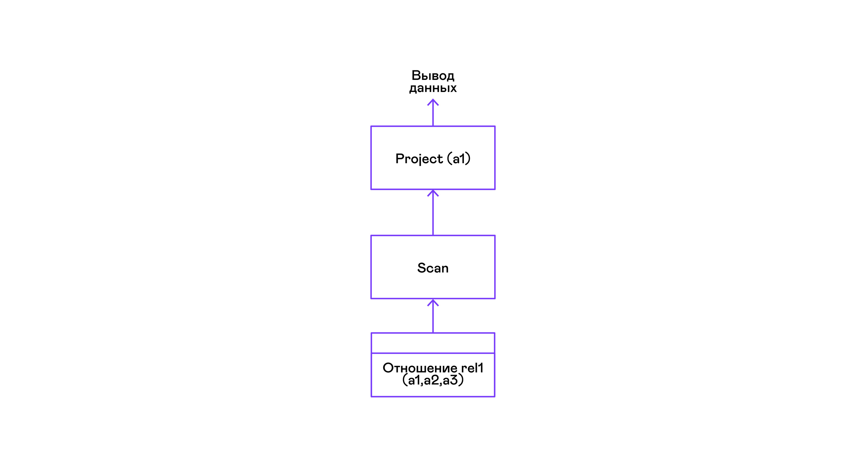
The simplest example where all tuples from a relation are selected:

 > ./pigletql > create table rel1 (a1,a2,a3); > insert into rel1 values (1,2,3); > insert into rel1 values (4,5,6); > select a1 from rel1; a1 1 4 rows: 2 > 

For the simplest of queries, only retrieving tuples from the scan relation are used, and selecting the only project attribute from the tuples:

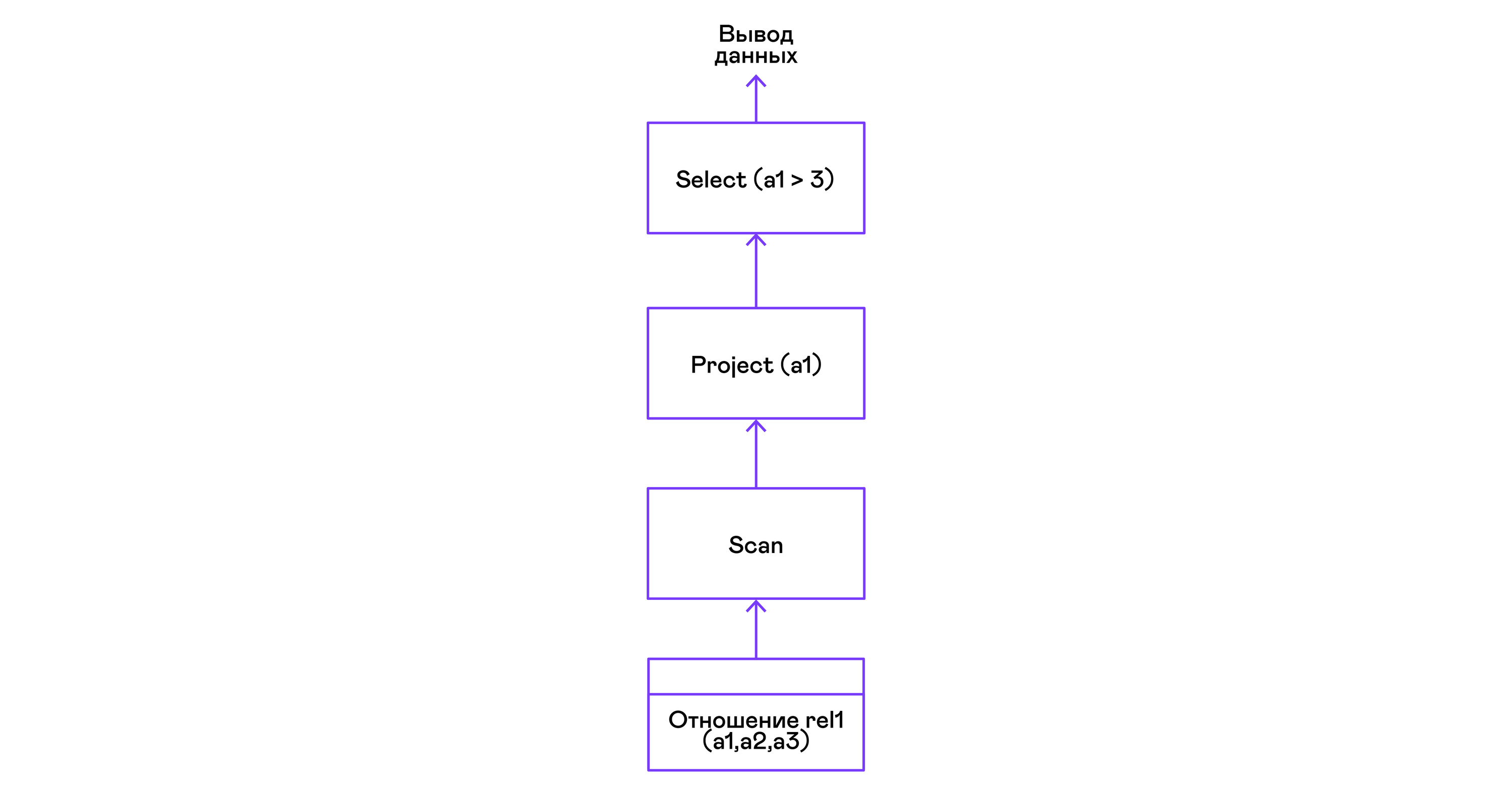
Choosing tuples with a predicate:

 > ./pigletql > create table rel1 (a1,a2,a3); > insert into rel1 values (1,2,3); > insert into rel1 values (4,5,6); > select a1 from rel1 where a1 > 3; a1 4 rows: 1 > 

Predicates are expressed by the select statement:

Selection of tuples with sorting:

 > ./pigletql > create table rel1 (a1,a2,a3); > insert into rel1 values (1,2,3); > insert into rel1 values (4,5,6); > select a1 from rel1 order by a1 desc; a1 4 1 rows: 2 

The scan sort operator in the open call creates ( materializes ) a temporary relationship, places all incoming tuples there, and sorts the whole. After that, in next calls, it infers tuples from the temporary relation in the order specified by the user:

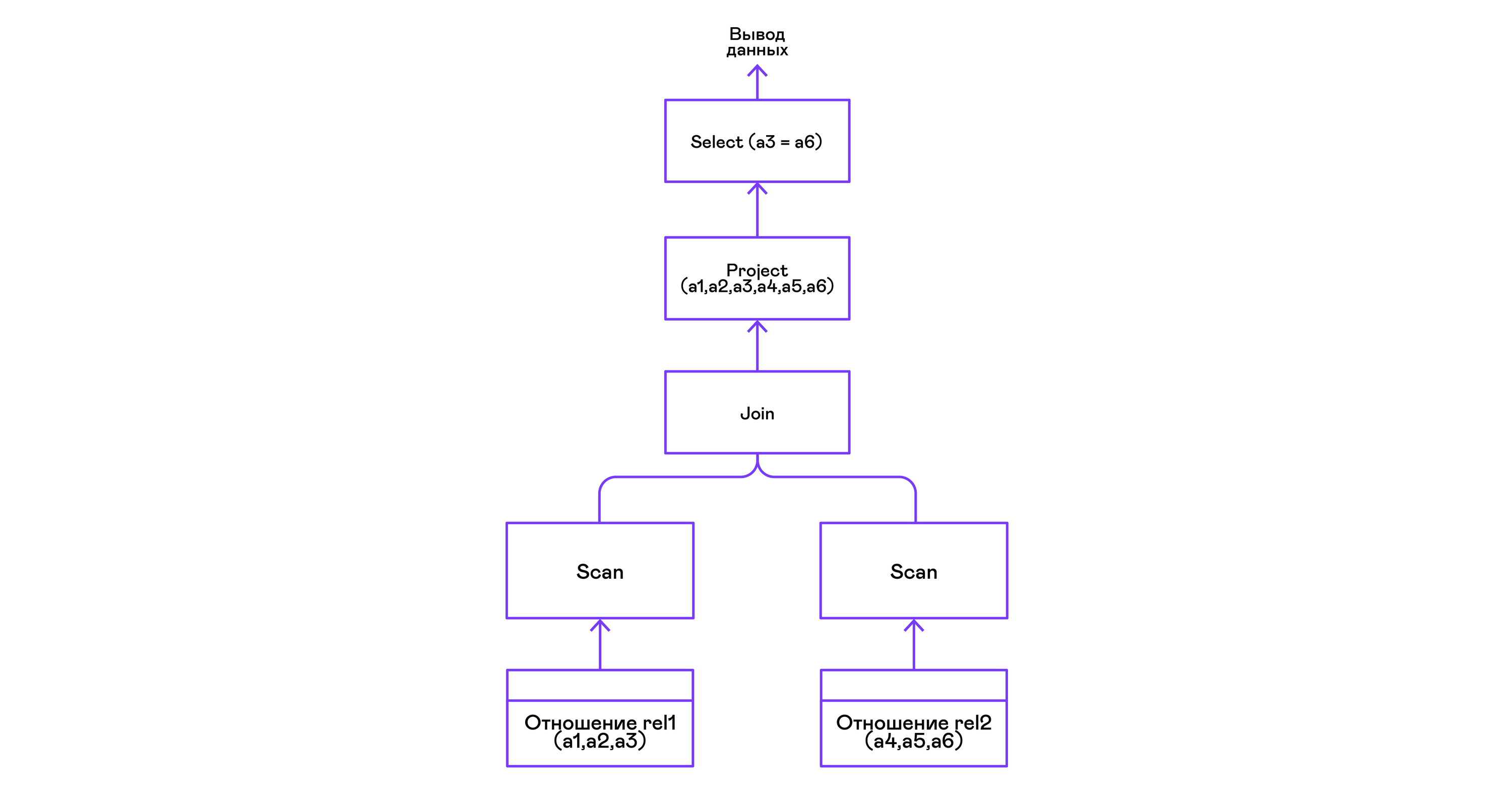
Combining tuples of two relations with a predicate:

 > ./pigletql > create table rel1 (a1,a2,a3); > insert into rel1 values (1,2,3); > insert into rel1 values (4,5,6); > create table rel2 (a4,a5,a6); > insert into rel2 values (7,8,6); > insert into rel2 values (9,10,6); > select a1,a2,a3,a4,a5,a6 from rel1, rel2 where a3=a6; a1 a2 a3 a4 a5 a6 4 5 6 7 8 6 4 5 6 9 10 6 rows: 2 

The join operator in PigletQL does not use any complex algorithms, but simply forms a Cartesian product from the sets of tuples of the left and right subtrees. This is very inefficient, but for a demo interpreter it will do:

findings

In conclusion, I note that if you are making an interpreter of a language similar to SQL, then you probably should just take any of the many available relational databases. Thousands of man-years have been invested in modern optimizers and query interpreters of popular databases, and it takes years to develop even the simplest general-purpose databases.

The demo language PigletQL imitates the work of the SQL interpreter, but in reality we use only individual elements of the Volcano architecture and only for those (rare!) Types of queries that are difficult to express in the framework of the relational model.

Nevertheless, I repeat: even a superficial acquaintance with the architecture of such interpreters is useful in cases where it is necessary to work flexibly with data streams.

Literature

If you are interested in the basic issues of database development, then books are better than “Database system implementation” (Garcia-Molina H., Ullman JD, Widom J., 2000), you will not find.

Its only drawback is a theoretical orientation. Personally, I like it when concrete examples of code or even a demo project are attached to the material. For this, you can refer to the book “Database design and implementation” (Sciore E., 2008), which provides the complete code for a relational database in Java.

The most popular relational databases still use variations on the Volcano theme. The original publication is written in a very accessible language and is easy to find on Google Scholar: “Volcano - an extensible and parallel query evaluation system” (Graefe G., 1994).

Although SQL interpreters have changed quite a bit in detail over the past decades, the very general structure of these systems has not changed for a very long time. You can get an idea of ​​it from a review paper by the same author, “Query evaluation techniques for large databases” (Graefe G. 1993).