Neural Networks and Deep Learning, Chapter 4: Visual Proof that Neural Networks Can Calculate Any Function
In this chapter, I give a simple and mostly visual explanation of the universality theorem. To follow the material in this chapter, you do not have to read the previous ones. It is structured as an independent essay. If you have the most basic understanding of NS, you should be able to understand the explanations.
One of the most amazing facts about neural networks is that they can calculate any function at all. That is, let's say that someone gives you some kind of complex and winding function f (x):

And regardless of this function, there is guaranteed such a neural network that for any input x the value f (x) (or some approximation close to it) will be the output of this network, that is:
')

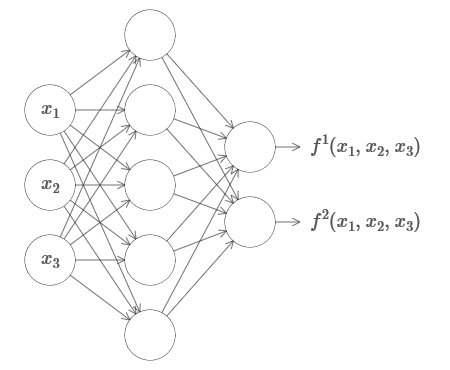
This works even if it is a function of many variables f = f (x 1 , ..., x m ), and with many values. For example, here is a network computing a function with m = 3 inputs and n = 2 outputs:
This result suggests that neural networks have a certain universality. No matter what function we want to calculate, we know that there is a neural network that can do this.
Moreover, the universality theorem holds even if we restrict the network to a single layer between incoming and outgoing neurons - the so-called in one hidden layer. So even networks with a very simple architecture can be extremely powerful.
The universality theorem is well known to people using neural networks. But although this is so, an understanding of this fact is not so widespread. And most of the explanations for this are too technically complex. For example, one of the first papers proving this result used the Hahn - Banach theorem , the Riesz representation theorem , and some Fourier analysis. If you are a mathematician, it’s easy for you to understand this evidence, but for most people it’s not so easy. It’s a pity, because the basic reasons for universality are simple and beautiful.
In this chapter, I give a simple and mostly visual explanation of the universality theorem. We will go step by step through the ideas underlying it. You will understand why neural networks can really calculate any function. You will understand some of the limitations of this result. And you will understand how the result is associated with deep NS.
To follow the material in this chapter, you do not have to read the previous ones. It is structured as an independent essay. If you have the most basic understanding of NS, you should be able to understand the explanations. But I will sometimes provide links to previous material to help fill knowledge gaps.
Universality theorems are often found in computer science, so sometimes we even forget how amazing they are. But it’s worth reminding yourself: the ability to calculate any arbitrary function is truly amazing. Almost any process that you can imagine can be reduced to calculating a function. Consider the task of finding the name of a musical composition based on a brief passage. This can be considered a function calculation. Or consider the task of translating a Chinese text into English. And this can be considered a function calculation (in fact, many functions, since there are many acceptable options for translating a single text). Or consider the task of generating a description of the plot of the film and the quality of the acting based on the mp4 file. This, too, can be considered as the calculation of a certain function (the remark made regarding the text translation options is also correct here). Universality means that, in principle, NSs can perform all these tasks, and many others.
Of course, only from the fact that we know that there are NSs capable of, say, translating from Chinese to English, it does not follow that we have good techniques for creating or even recognizing such a network. This restriction also applies to traditional universality theorems for models such as Boolean schemes. But, as we have already seen in this book, the NS has powerful algorithms for learning functions. The combination of learning algorithms and versatility is an attractive mix. So far in the book, we have focused on training algorithms. In this chapter, we will focus on universality and what it means.
Before explaining why the universality theorem is true, I want to mention two tricks contained in the informal statement “a neural network can calculate any function”.
Firstly, this does not mean that the network can be used to accurately calculate any function. We can only get as good an approximation as we need. By increasing the number of hidden neurons, we improve the approximation. For example, I previously illustrated a network computing a certain function f (x) using three hidden neurons. For most functions, using three neurons, only a low-quality approximation can be obtained. By increasing the number of hidden neurons (say, up to five), we can usually get an improved approximation:
And to improve the situation, increasing the number of hidden neurons and further.
To clarify this statement, let's say we were given a function f (x), which we want to calculate with some necessary accuracy ε> 0. There is a guarantee that when using a sufficient number of hidden neurons, we can always find an NS whose output g (x) satisfies the equation | g (x) −f (x) | <ε for any x. In other words, the approximation will be achieved with the desired accuracy for any possible input value.
The second catch is that functions that can be approximated by the described method belong to a continuous class. If the function is interrupted, that is, it makes sudden sharp jumps, then in the general case it will be impossible to approximate with the help of NS. And this is not surprising, since our NSs calculate continuous functions of input data. However, even if the function that we really need to calculate is discontinuous, the approximation is often quite continuous. If so, then we can use NS. In practice, this limitation is usually not important.
As a result, a more accurate statement of the universality theorem will be that NS with one hidden layer can be used to approximate any continuous function with any desired accuracy. In this chapter, we prove a slightly less rigorous version of this theorem, using two hidden layers instead of one. In tasks, I will briefly describe how this explanation can, with minor modifications, be adapted to a proof that uses only one hidden layer.
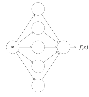
To understand why the universality theorem is true, we begin by understanding how to create an NS approximating function with only one input and one output value:
It turns out that this is the essence of the task of universality. Once we understand this special case, it will be quite easy to extend it to functions with many input and output values.
To create an understanding of how to construct a network for counting f, we start with a network containing a single hidden layer with two hidden neurons, and with an output layer containing one output neuron:

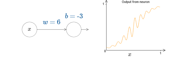
To imagine how the network components work, we focus on the upper hidden neuron. In the diagram in the original article, you can interactively change the weight with the mouse by clicking on “w” and immediately see how the function calculated by the upper hidden neuron changes:

As we learned earlier in the book, a hidden neuron counts σ (wx + b), where σ (z) ≡ 1 / (1 + e −z ) is a sigmoid . So far, we have used this algebraic form quite often. However, to prove universality it would be better if we completely ignore this algebra, and instead manipulate and observe the shape on the graph. This will not only help you better feel what is happening, but also give us a proof of universality applicable to other activation functions besides sigmoid.
Strictly speaking, the visual approach I have chosen is traditionally not considered evidence. But I believe that the visual approach provides more insight into the truth of the final result than traditional proof. And, of course, such an understanding is the real purpose of the proof. In the evidence I propose, gaps will occasionally come across; I will give reasonable, but not always rigorous visual evidence. If this bothers you, then consider it your task to fill these gaps. However, do not lose sight of the main goal: to understand why the universality theorem is true.
To begin with this proof, click on the offset b in the original diagram and drag to the right to enlarge it. You will see that with increasing displacement, the graph moves to the left, but does not change shape.
Then drag it to the left to reduce the offset. You will see that the graph is moving to the right without changing shape.
Reduce weight to 2-3. You will see that as the weight decreases, the curve straightens. To prevent the curve from running off the graph, you may need to correct the offset.
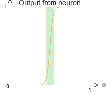
Finally, increase the weight to values greater than 100. The curve will become steeper, and eventually approach the step. Try adjusting the offset so that its angle is in the region of the point x = 0.3. The video below shows what should happen:
We can greatly simplify our analysis by increasing the weight so that the output is really a good approximation of the step function. Below I built the output of the upper hidden neuron for the weight w = 999. This is a static image:
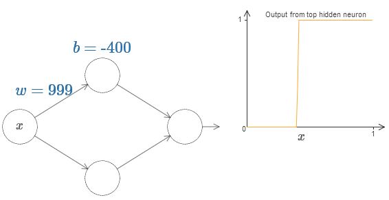
Using step functions is a bit easier than with typical sigmoid. The reason is that contributions from all hidden neurons are added up in the output layer. The sum of a bunch of step functions is easy to analyze, but it’s more difficult to talk about what happens when a bunch of curves are added in the form of a sigmoid. Therefore, it will be much easier to assume that our hidden neurons produce stepwise functions. More precisely, we do this by fixing the weight w at some very large value, and then assigning the position of the step through the offset. Of course, working with an output as a step function is an approximation, but it is very good, and so far we will treat the function as a true step function. Later, I will return to a discussion of the effect of deviations from this approximation.
What value of x is the step? In other words, how does the position of the step depend on weight and displacement?
To answer the question, try changing the weight and offset in the interactive chart. Can you understand how the position of a step depends on w and b? By practicing a little, you can convince yourself that its position is proportional to b and inversely proportional to w.
In fact, the step is at s = −b / w, as will be seen if we adjust the weight and displacement to the following values:
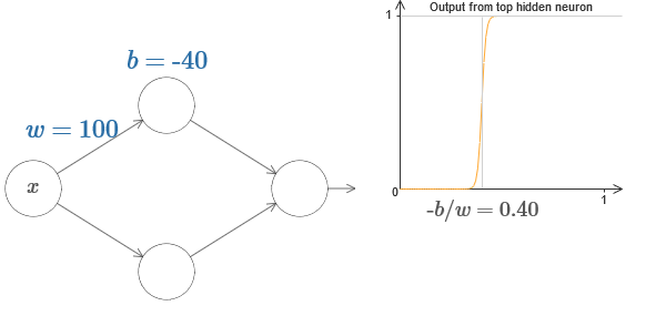
Our lives will be greatly simplified if we describe hidden neurons with a single parameter, s, that is, by the position of the step, s = −b / w. In the following interactive diagram, you can simply change s:

As noted above, we specially assigned a weight w at the input to a very large value - large enough so that the step function becomes a good approximation. And we can easily turn the parameterized neuron in this way back to its usual form by choosing the bias b = −ws.
So far, we have concentrated on the output of only the superior hidden neuron. Let's look at the behavior of the entire network. Suppose that hidden neurons calculate the step functions defined by the parameters of the steps s 1 (upper neuron) and s 2 (lower neuron). Their respective output weights are w 1 and w 2 . Here is our network:
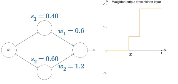
On the right is a graph of the weighted output w 1 a 1 + w 2 a 2 of the hidden layer. Here a 1 and a 2 are the outputs of the upper and lower hidden neurons, respectively. They are denoted by “a”, as they are often called neuronal activations.
By the way, we note that the output of the entire network is σ (w 1 a 1 + w 2 a 2 + b), where b is the bias of the output neuron. This, obviously, is not the same as the weighted output of the hidden layer whose graph we are building. But for now, we will concentrate on the balanced output of the hidden layer, and only later think about how it relates to the output of the entire network.
Try to increase and decrease the step s 1 of the upper hidden neuron on the interactive diagram in the original article . See how this changes the weighted output of the hidden layer. It is especially useful to understand what happens when s 1 exceeds s 2 . You will see that the graph in these cases changes shape, as we move from a situation in which the upper hidden neuron is activated first to a situation in which the lower hidden neuron is activated first.
Similarly, try manipulating the s 2 step of the lower hidden neuron and see how this changes the overall output of the hidden neurons.
Try to reduce and increase output weights. Notice how this scales the contribution from the corresponding hidden neurons. What happens if one of the weights equals 0?
Finally, try setting w 1 to 0.8 and w 2 to -0.8. The result is a “protrusion” function, with a start at s 1 , an end at s 2 , and a height of 0.8. For example, a weighted output might look like this:
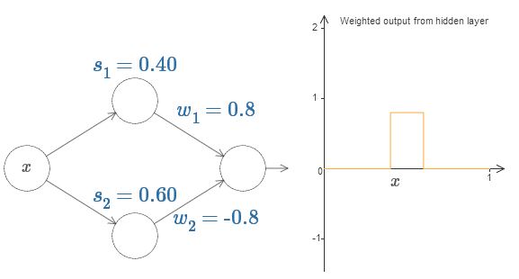
Of course, the protrusion can be scaled to any height. Let's use one parameter, h, denoting height. Also, for simplicity, I will get rid of the notation "s 1 = ..." and "w 1 = ...".
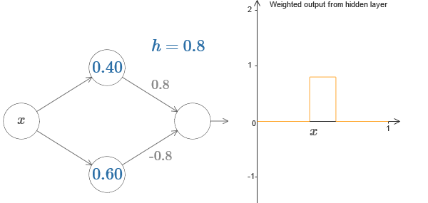
Try increasing and decreasing the h value to see how the height of the protrusion changes. Try to make h negative. Try changing the points of the steps to observe how this changes the shape of the protrusion.
You will see that we use our neurons not just as graphic primitives, but also as units more familiar to programmers - something like an if-then-else instruction in programming:
if input> = start of step:
add 1 to weighted output
else:
add 0 to weighted output
For the most part I will stick to the graphic notation. However, sometimes it will be useful for you to switch to the if-then-else view and reflect on what is happening in these terms.
We can use our protrusion trick by gluing two parts of hidden neurons together on the same network:
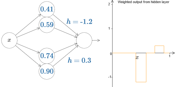
Here I dropped the weights by simply writing down the h values for each pair of hidden neurons. Try playing with both h values and see how it changes the graph. Move the tabs, changing the points of the steps.
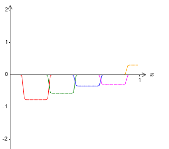
In a more general case, this idea can be used to obtain any desired number of peaks of any height. In particular, we can divide the interval [0,1] into a large number of (N) subintervals, and use N pairs of hidden neurons to obtain peaks of any desired height. Let's see how this works for N = 5. This is already quite a lot of neurons, so I'm a little narrower representation. Sorry for the complicated diagram - I could hide the complexity behind additional abstractions, but it seems to me that it is worth a little torment with the complexity in order to better feel how the neural networks work.
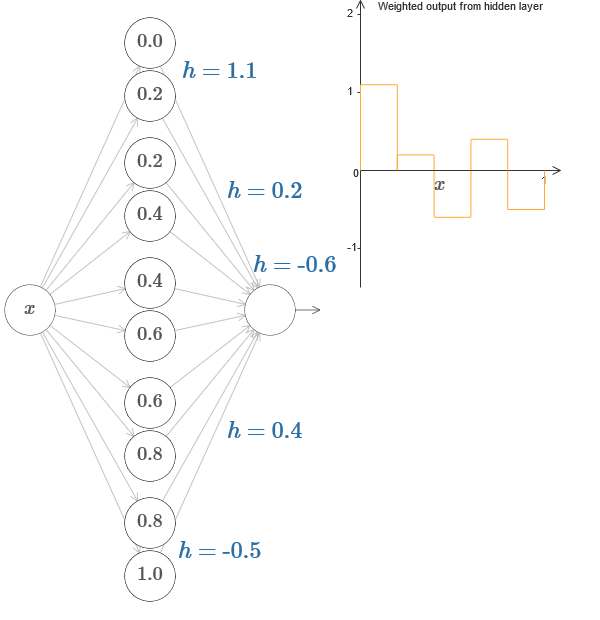
You see, we have five pairs of hidden neurons. The points of the steps of the corresponding pairs are located at 0.1 / 5, then 1 / 5.2 / 5, and so on, up to 4 / 5.5 / 5. These values are fixed - we get five protrusions of equal width on the graph.
Each pair of neurons has a value h associated with it. Remember that neuron output links have weights h and –h. In the original article in the diagram, you can click on the h values and move them left-right. With a change in height, the schedule also changes. By changing the output weights, we construct the final function!
On the diagram, you can still click on the graph, and drag the height of the steps up or down. When you change its height, you see how the height of the corresponding h changes. The output weights + h and –h change accordingly. In other words, we directly manipulate a function whose graph is shown on the right and see these changes in the values of h on the left. You can also hold down the mouse button on one of the protrusions, and then drag the mouse left or right, and the protrusions will adjust to the current height.
It is time to get the job done.
Recall the function that I drew at the very beginning of the chapter:
Then I did not mention this, but in fact it looks like this:
It is constructed for x values from 0 to 1, and values along the y axis vary from 0 to 1.
Obviously, this function is nontrivial. And you have to figure out how to calculate it using neural networks.
In our neural networks above, we analyzed a weighted combination ∑ j w j a j of the output of hidden neurons. We know how to get significant control over this value. But, as I noted earlier, this value is not equal to the network output. The network output is σ (∑ j w j a j + b), where b is the bias of the output neuron. Can we gain control directly over the network output?
The solution is to develop a neural network in which the weighted output of the hidden layer is given by the equation σ −1 ⋅f (x), where σ −1 is the inverse function of σ. That is, we want the weighted output of the hidden layer to be like this:
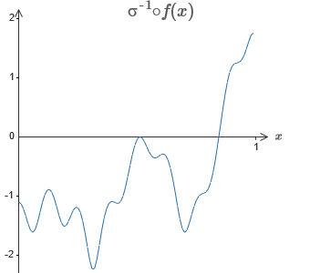
If this succeeds, then the output of the entire network will be a good approximation of f (x) (I set the offset of the output neuron to 0).
Then your task is to develop an NS approximating the objective function shown above. To better understand what is happening, I recommend that you solve this problem twice. For the first time in the original article, click on the graph, and directly adjust the heights of the different protrusions. It will be quite easy for you to get a good approximation to the objective function. The degree of approximation is estimated by the average deviation, the difference between the objective function and the function that the network calculates. Your task is to bring the average deviation to a minimum value. The task is considered completed when the average deviation does not exceed 0.40.
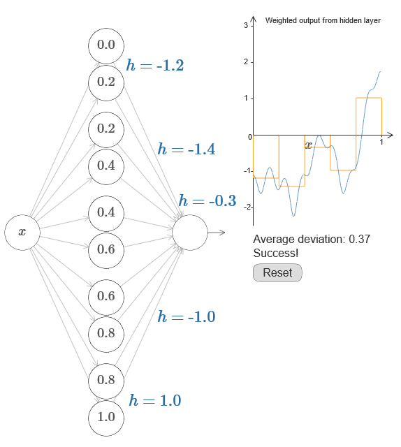
Once successful, press the Reset button, which randomly changes the tabs. The second time, do not touch the graph, but change the h values on the left side of the diagram, trying to bring the average deviation to a value of 0.40 or less.
And so, you have found all the elements necessary for the network to approximately calculate the function f (x)! The approximation turned out to be rough, but we can easily improve the result by simply increasing the number of pairs of hidden neurons, which will increase the number of protrusions.
In particular, it is easy to turn all the data found back into the standard view with parameterization used for NS. Let me quickly remind you how this works.
In the first layer, all weights have a large constant value, for example, w = 1000.
The displacements of hidden neurons are calculated through b = −ws. So, for example, for the second hidden neuron, s = 0.2 turns into b = −1000 × 0.2 = −200.
The last layer of the scale is determined by the values of h. So, for example, the value you choose for the first h, h = -0.2, means that the output weights of the two upper hidden neurons are -0.2 and 0.2, respectively. And so on, for the entire output weight layer.
Finally, the offset of the output neuron is 0.
And that’s all: we got a complete description of the NS, which calculates the initial objective function well. And we understand how to improve the quality of approximation by improving the number of hidden neurons.
In addition, in our original objective function f (x) = 0.2 + 0.4x 2 + 0.3sin (15x) + 0.05cos (50x) there is nothing special. A similar procedure could be used for any continuous function on the intervals from [0,1] to [0,1]. In fact, we use our single-layer NS to build a lookup table for the function. And we can take this idea as a basis to get a generalized proof of universality.
We extend our results to the case of a set of input variables. It sounds complicated, but all the ideas we need can already be understood for the case with only two incoming variables. Therefore, we consider the case with two incoming variables.
Let's start by looking at what will happen when a neuron has two inputs:
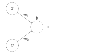
We have inputs x and y, with corresponding weights w 1 and w 2 and offset b of the neuron. Set the weight of w 2 to 0 and play with the first one, w 1 , and offset b to see how they affect the output of the neuron:
As you can see, with w 2 = 0, the input y does not affect the output of the neuron. Everything happens as if x is the only input.
Given this, what do you think will happen when we increase the weight of w 1 to w 1 = 100 and w 2 leave 0? If this is not immediately clear to you, think a little about this issue. Then watch the following video, which shows what will happen:
As before, with an increase in the input weight, the output approaches the shape of the step. The difference is that our step function is now located in three dimensions. As before, we can move the location of the steps by changing the offset. The angle will be at the point s x ≡ − b / w1.
Let's redo the diagram so that the parameter is the location of the step:
We assume that the input weight of x is of great importance - I used w 1 = 1000 - and the weight of w 2 = 0. The number on the neuron is the position of the step, and the x above it reminds us that we move the step along the x axis. Naturally, it is quite possible to obtain a step function along the y axis, making the incoming weight for y large (say, w 2 = 1000), and the weight for x equal to 0, w 1 = 0:
The number on the neuron, again, indicates the position of the step, and the y above it reminds us that we move the step along the y axis. I could directly designate the weights for x and y, but I didn’t, because that would litter the chart. But keep in mind that the y marker indicates that the weight for y is large and for x is 0.
We can use the step functions we have just designed to calculate the three-dimensional protrusion function. To do this, we take two neurons, each of which will calculate a step function along the x axis. Then we combine these step functions with weights h and –h, where h is the desired height of the protrusion.All this can be seen in the following diagram:
Try changing the value of h. See how it relates to network weights. And how she changes the height of the protrusion function on the right.
Also try to change the point of the step, the value of which is set to 0.30 in the upper hidden neuron. See how it changes the shape of the protrusion. What happens if we move it beyond the 0.70 point associated with the lower hidden neuron?
We learned how to build the protrusion function along the x axis. Naturally, we can easily make the protrusion function along the y axis, using two step functions along the y axis. Recall that we can do this by making large weights at input y and setting weight 0 at input x. And so, what happens:
It looks almost identical to the previous network! The only visible change is small y markers on hidden neurons. They remind us that they produce step functions for y, and not for x, so at the input y the weight is very large and at the input x it is zero, and not vice versa. As before, I decided not to show it directly, so as not to clutter up the picture.
Let's see what happens if we add two protrusion functions, one along the x axis, the other along the y axis, both of height h:

To simplify the connection diagram with zero weight, I omitted. So far, I have left small x and y markers on hidden neurons to recall in which directions the protrusion functions are computed. Later we will refuse them, since they are implied by the incoming variable.
Try changing the parameter h. As you can see, because of this, the output weights change, as well as the weights of both protrusion functions, x and y.
What we created is a bit like a “tower function”:
If we can create such tower functions, we can use them to approximate arbitrary functions by simply adding towers of different heights in different places:
Of course, we have not yet reached the creation of an arbitrary tower function. So far we have constructed something like a central tower of height 2h with a plateau of height h surrounding it.
But we can make a tower function. Recall that we previously showed how neurons can be used to implement the if-then-else statement:
It was a one-input neuron. And we need to apply a similar idea to the combined output of hidden neurons:
If we choose the right threshold - for example, 3h / 2, squeezed between the height of the plateau and the height of the central tower - we can crush the plateau to zero, and leave only one tower.
Imagine how to do this? Try experimenting with the following network. Now we are plotting the output of the entire network, and not just the weighted output of the hidden layer. This means that we add the offset term to the weighted output from the hidden layer, and apply the sigmoid. Can you find the values for h and b for which you get a tower? If you get stuck at this point, here are two tips: (1) for the outgoing neuron to show the correct behavior in the if-then-else style, we need the incoming weights (all h or –h) to be large; (2) the value of b determines the scale of the if-then-else threshold.
With default parameters, the output is similar to a flattened version of the previous diagram, with a tower and plateau. To get the desired behavior, you need to increase the value of h. This will give us threshold if-then-else behavior. Secondly, in order to set the threshold correctly, one must choose b ≈ −3h / 2.
Here's what it looks like for h = 10:
Even for relatively modest values of h, we get a nice tower function. And, of course, we can get an arbitrarily beautiful result by increasing h further and keeping the displacement at the level b = −3h / 2.
Let's try to glue two networks together to count two different tower functions. To make the respective roles of the two subnets clear, I put them in separate rectangles: each of them calculates the tower function using the technique described above. The graph on the right shows the weighted output of the second hidden layer, that is, the weighted combination of tower functions.
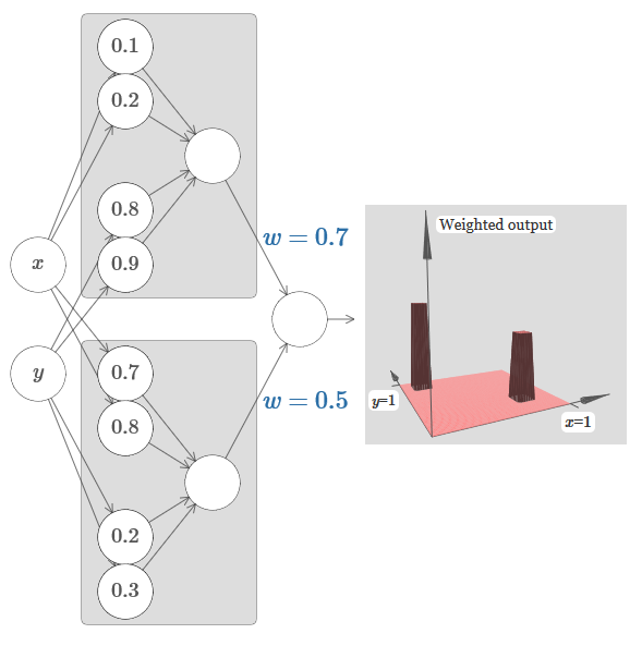
In particular, it can be seen that by changing the weights in the last layer, you can change the height of the output towers.
The same idea allows you to calculate as many towers as you like. We can make them arbitrarily thin and tall. As a result, we guarantee that the weighted output of the second hidden layer approximates any desired function of two variables:
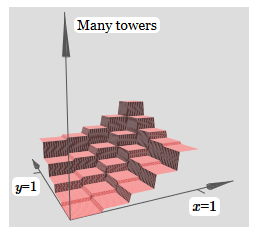
In particular, by making the weighted output of the second hidden layer approximate σ −1 ⋅f well, we guarantee that the output of our network will be a good approximation of the desired function f.
What about the functions of many variables?
Let's try to take three variables, x 1 , x 2 , x 3 . Can the following network be used to calculate the tower function in four dimensions?
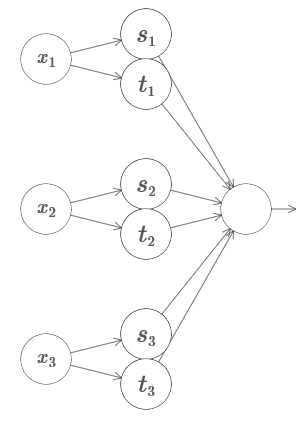
Here x 1 , x 2 , x 3 denote the network input. s 1 , t 1, and so on - step points for neurons - that is, all the weights in the first layer are large, and the offsets are assigned so that the points of the steps are s 1 , t 1 , s 2 , ... The weights in the second layer alternate, + h, −h, where h is some very large number. The output offset is −5h / 2.
The network computes a function equal to 1 under three conditions: x 1 is between s 1 and t 1 ; x 2 is between s 2 and t 2 ; x 3 is between s 3 and t 3 . The network is 0 in all other places. This is such a tower, in which 1 is a small portion of the entrance space, and 0 is everything else.
Gluing a lot of such networks, we can get as many towers as we like, and approximate an arbitrary function of three variables. The same idea works in m dimensions. Only the output offset (−m + 1/2) h is changed to properly squeeze the desired values and remove the plateau.
Well, now we know how to use NS to approximate the real function of many variables. What about vector functions f (x 1 , ..., x m ) ∈ R n ? Of course, such a function can be considered simply as n separate real functions f1 (x 1 , ..., x m ), f2 (x 1 , ..., x m ), and so on. And then we just glue all the networks together. So it's easy to figure it out.
We have proven that a network of sigmoid neurons can calculate any function. Recall that in a sigmoid neuron, the inputs x 1 , x 2 , ... turn at the output into σ (∑ j w j x j j + b), where w j are the weights, b is the bias, and σ is the sigmoid.

What if we look at another type of neuron using a different activation function, s (z):
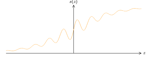
That is, we will assume that if a neuron has x 1 , x 2 , ... weights w 1 , w 2 , ... and bias b, then s (∑ j w j x j + b) will be output.
We can use this activation function to get stepped, just like in the case of the sigmoid. Try (in the original article ) on the diagram to lift up the weight to, say, w = 100:

As in the case of the sigmoid, because of this, the activation function is compressed, and as a result turns into a very good approximation of the step function. Try changing the offset, and you will see that we can change the location of the step to any. Therefore, we can use all the same tricks as before to calculate any desired function.
What properties should s (z) have in order for this to work? We need to assume that s (z) is well defined as z → −∞ and z → ∞. These limits are two values accepted by our step function. We also need to assume that these limits are different. If they didn’t differ, the steps would not work; there would simply be a flat schedule! But if the activation function s (z) satisfies these properties, the neurons based on it are universally suitable for calculations.
For the time being, we assumed that our neurons produce accurate step functions. This is a good approximation, but only an approximation. In fact, there is a narrow gap of failure, shown in the following graph, where the functions do not behave at all like a step function:
In this period of failure, my explanation of universality does not work.
Failure is not so scary. By setting sufficiently large input weights, we can make these gaps arbitrarily small. We can make them much smaller than on the chart, invisible to the eye. So maybe we don’t have to worry about this problem.
Nevertheless, I would like to have some way to solve it.
It turns out that it’s easy to solve. Let’s look at this solution for calculating NS functions with only one input and output. The same ideas will work to solve the problem with a large number of inputs and outputs.
In particular, let's say we want our network to compute some function f. As before, we try to do this by designing the network so that the weighted output of the hidden layer of neurons is σ −1 ⋅f (x):
If we do this using the technique described above, we will make the hidden neurons give out a sequence of functions of the protrusions:
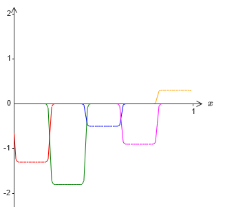
Of course, I exaggerated the size of the intervals of failure, so that they were easier to see. It should be clear that if we add up all these functions of the protrusions, we get a fairly good approximation of σ −1 ⋅f (x) everywhere except for the intervals of failure.
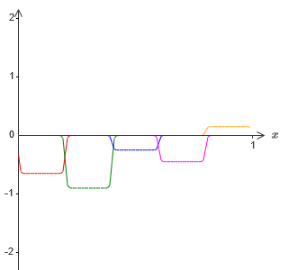
But, suppose that instead of using the approximation just described, we use a set of hidden neurons to calculate the approximation of half of our original objective function, i.e., σ −1 ⋅f (x) / 2. Of course, it will look just like a scaled version of the latest graph:
And suppose we make one more set of hidden neurons calculate the approximation to σ −1 ⋅f (x) / 2, however, at its base the protrusions will be shifted by half their width:
Now we have two different approximations for σ − 1⋅f (x) / 2. If we add up these two approximations, we obtain a general approximation to σ − 1⋅f (x). This general approximation will still have inaccuracies in small intervals. But the problem will be less than before - because the points falling into the intervals of the failure of the first approximation will not fall into the intervals of the failure of the second approximation. Therefore, the approximation in these intervals will be approximately 2 times better.
We can improve the situation by adding a large number, M, of overlapping approximations of the function σ − 1⋅f (x) / M. If all of their failure intervals are narrow enough, any current will be in only one of them. If you use a sufficiently large number of overlapping approximations of M, the result will be an excellent general approximation.
The explanation of universality discussed here definitely cannot be called a practical description of how to count functions using neural networks! In this sense, it is more like proof of the versatility of NAND logic gates and more. Therefore, I basically tried to make this design clear and easy to follow without optimizing its details. However, trying to optimize this design can be an interesting and instructive exercise for you.
Although the result obtained cannot be directly used to create NS, it is important because it removes the question of the computability of any particular function using NS. The answer to such a question will always be positive. Therefore, it is correct to ask if any function is computable, but what is the correct way to calculate it.
Our universal design uses only two hidden layers to calculate an arbitrary function. As we discussed, it is possible to get the same result with a single hidden layer. Given this, you may wonder why we need deep networks, that is, networks with a large number of hidden layers. Can't we just replace these networks with shallow ones that have one hidden layer?
Although, in principle, it is possible, there are good practical reasons for using deep neural networks. As described in Chapter 1, deep NSs have a hierarchical structure that allows them to adapt well to study hierarchical knowledge, which are useful for solving real problems. More specifically, when solving problems such as pattern recognition, it is useful to use a system that understands not only individual pixels, but also increasingly complex concepts: from borders to simple geometric shapes, and beyond, to complex scenes involving several objects. In later chapters we will see evidence in favor of the fact that deep NSs will be better able to cope with the study of such hierarchies of knowledge than shallow ones. To summarize: universality tells us that NS can calculate any function; empirical evidence suggests that deep NSs are better adapted to the study of functions useful for solving many real-world problems.
Content
One of the most amazing facts about neural networks is that they can calculate any function at all. That is, let's say that someone gives you some kind of complex and winding function f (x):
And regardless of this function, there is guaranteed such a neural network that for any input x the value f (x) (or some approximation close to it) will be the output of this network, that is:
')
This works even if it is a function of many variables f = f (x 1 , ..., x m ), and with many values. For example, here is a network computing a function with m = 3 inputs and n = 2 outputs:
This result suggests that neural networks have a certain universality. No matter what function we want to calculate, we know that there is a neural network that can do this.
Moreover, the universality theorem holds even if we restrict the network to a single layer between incoming and outgoing neurons - the so-called in one hidden layer. So even networks with a very simple architecture can be extremely powerful.
The universality theorem is well known to people using neural networks. But although this is so, an understanding of this fact is not so widespread. And most of the explanations for this are too technically complex. For example, one of the first papers proving this result used the Hahn - Banach theorem , the Riesz representation theorem , and some Fourier analysis. If you are a mathematician, it’s easy for you to understand this evidence, but for most people it’s not so easy. It’s a pity, because the basic reasons for universality are simple and beautiful.
In this chapter, I give a simple and mostly visual explanation of the universality theorem. We will go step by step through the ideas underlying it. You will understand why neural networks can really calculate any function. You will understand some of the limitations of this result. And you will understand how the result is associated with deep NS.
To follow the material in this chapter, you do not have to read the previous ones. It is structured as an independent essay. If you have the most basic understanding of NS, you should be able to understand the explanations. But I will sometimes provide links to previous material to help fill knowledge gaps.
Universality theorems are often found in computer science, so sometimes we even forget how amazing they are. But it’s worth reminding yourself: the ability to calculate any arbitrary function is truly amazing. Almost any process that you can imagine can be reduced to calculating a function. Consider the task of finding the name of a musical composition based on a brief passage. This can be considered a function calculation. Or consider the task of translating a Chinese text into English. And this can be considered a function calculation (in fact, many functions, since there are many acceptable options for translating a single text). Or consider the task of generating a description of the plot of the film and the quality of the acting based on the mp4 file. This, too, can be considered as the calculation of a certain function (the remark made regarding the text translation options is also correct here). Universality means that, in principle, NSs can perform all these tasks, and many others.
Of course, only from the fact that we know that there are NSs capable of, say, translating from Chinese to English, it does not follow that we have good techniques for creating or even recognizing such a network. This restriction also applies to traditional universality theorems for models such as Boolean schemes. But, as we have already seen in this book, the NS has powerful algorithms for learning functions. The combination of learning algorithms and versatility is an attractive mix. So far in the book, we have focused on training algorithms. In this chapter, we will focus on universality and what it means.
Two tricks
Before explaining why the universality theorem is true, I want to mention two tricks contained in the informal statement “a neural network can calculate any function”.
Firstly, this does not mean that the network can be used to accurately calculate any function. We can only get as good an approximation as we need. By increasing the number of hidden neurons, we improve the approximation. For example, I previously illustrated a network computing a certain function f (x) using three hidden neurons. For most functions, using three neurons, only a low-quality approximation can be obtained. By increasing the number of hidden neurons (say, up to five), we can usually get an improved approximation:
And to improve the situation, increasing the number of hidden neurons and further.
To clarify this statement, let's say we were given a function f (x), which we want to calculate with some necessary accuracy ε> 0. There is a guarantee that when using a sufficient number of hidden neurons, we can always find an NS whose output g (x) satisfies the equation | g (x) −f (x) | <ε for any x. In other words, the approximation will be achieved with the desired accuracy for any possible input value.
The second catch is that functions that can be approximated by the described method belong to a continuous class. If the function is interrupted, that is, it makes sudden sharp jumps, then in the general case it will be impossible to approximate with the help of NS. And this is not surprising, since our NSs calculate continuous functions of input data. However, even if the function that we really need to calculate is discontinuous, the approximation is often quite continuous. If so, then we can use NS. In practice, this limitation is usually not important.
As a result, a more accurate statement of the universality theorem will be that NS with one hidden layer can be used to approximate any continuous function with any desired accuracy. In this chapter, we prove a slightly less rigorous version of this theorem, using two hidden layers instead of one. In tasks, I will briefly describe how this explanation can, with minor modifications, be adapted to a proof that uses only one hidden layer.
Versatility with one input and one output value
To understand why the universality theorem is true, we begin by understanding how to create an NS approximating function with only one input and one output value:
It turns out that this is the essence of the task of universality. Once we understand this special case, it will be quite easy to extend it to functions with many input and output values.
To create an understanding of how to construct a network for counting f, we start with a network containing a single hidden layer with two hidden neurons, and with an output layer containing one output neuron:
To imagine how the network components work, we focus on the upper hidden neuron. In the diagram in the original article, you can interactively change the weight with the mouse by clicking on “w” and immediately see how the function calculated by the upper hidden neuron changes:
As we learned earlier in the book, a hidden neuron counts σ (wx + b), where σ (z) ≡ 1 / (1 + e −z ) is a sigmoid . So far, we have used this algebraic form quite often. However, to prove universality it would be better if we completely ignore this algebra, and instead manipulate and observe the shape on the graph. This will not only help you better feel what is happening, but also give us a proof of universality applicable to other activation functions besides sigmoid.
Strictly speaking, the visual approach I have chosen is traditionally not considered evidence. But I believe that the visual approach provides more insight into the truth of the final result than traditional proof. And, of course, such an understanding is the real purpose of the proof. In the evidence I propose, gaps will occasionally come across; I will give reasonable, but not always rigorous visual evidence. If this bothers you, then consider it your task to fill these gaps. However, do not lose sight of the main goal: to understand why the universality theorem is true.
To begin with this proof, click on the offset b in the original diagram and drag to the right to enlarge it. You will see that with increasing displacement, the graph moves to the left, but does not change shape.
Then drag it to the left to reduce the offset. You will see that the graph is moving to the right without changing shape.
Reduce weight to 2-3. You will see that as the weight decreases, the curve straightens. To prevent the curve from running off the graph, you may need to correct the offset.
Finally, increase the weight to values greater than 100. The curve will become steeper, and eventually approach the step. Try adjusting the offset so that its angle is in the region of the point x = 0.3. The video below shows what should happen:
We can greatly simplify our analysis by increasing the weight so that the output is really a good approximation of the step function. Below I built the output of the upper hidden neuron for the weight w = 999. This is a static image:
Using step functions is a bit easier than with typical sigmoid. The reason is that contributions from all hidden neurons are added up in the output layer. The sum of a bunch of step functions is easy to analyze, but it’s more difficult to talk about what happens when a bunch of curves are added in the form of a sigmoid. Therefore, it will be much easier to assume that our hidden neurons produce stepwise functions. More precisely, we do this by fixing the weight w at some very large value, and then assigning the position of the step through the offset. Of course, working with an output as a step function is an approximation, but it is very good, and so far we will treat the function as a true step function. Later, I will return to a discussion of the effect of deviations from this approximation.
What value of x is the step? In other words, how does the position of the step depend on weight and displacement?
To answer the question, try changing the weight and offset in the interactive chart. Can you understand how the position of a step depends on w and b? By practicing a little, you can convince yourself that its position is proportional to b and inversely proportional to w.
In fact, the step is at s = −b / w, as will be seen if we adjust the weight and displacement to the following values:
Our lives will be greatly simplified if we describe hidden neurons with a single parameter, s, that is, by the position of the step, s = −b / w. In the following interactive diagram, you can simply change s:
As noted above, we specially assigned a weight w at the input to a very large value - large enough so that the step function becomes a good approximation. And we can easily turn the parameterized neuron in this way back to its usual form by choosing the bias b = −ws.
So far, we have concentrated on the output of only the superior hidden neuron. Let's look at the behavior of the entire network. Suppose that hidden neurons calculate the step functions defined by the parameters of the steps s 1 (upper neuron) and s 2 (lower neuron). Their respective output weights are w 1 and w 2 . Here is our network:
On the right is a graph of the weighted output w 1 a 1 + w 2 a 2 of the hidden layer. Here a 1 and a 2 are the outputs of the upper and lower hidden neurons, respectively. They are denoted by “a”, as they are often called neuronal activations.
By the way, we note that the output of the entire network is σ (w 1 a 1 + w 2 a 2 + b), where b is the bias of the output neuron. This, obviously, is not the same as the weighted output of the hidden layer whose graph we are building. But for now, we will concentrate on the balanced output of the hidden layer, and only later think about how it relates to the output of the entire network.
Try to increase and decrease the step s 1 of the upper hidden neuron on the interactive diagram in the original article . See how this changes the weighted output of the hidden layer. It is especially useful to understand what happens when s 1 exceeds s 2 . You will see that the graph in these cases changes shape, as we move from a situation in which the upper hidden neuron is activated first to a situation in which the lower hidden neuron is activated first.
Similarly, try manipulating the s 2 step of the lower hidden neuron and see how this changes the overall output of the hidden neurons.
Try to reduce and increase output weights. Notice how this scales the contribution from the corresponding hidden neurons. What happens if one of the weights equals 0?
Finally, try setting w 1 to 0.8 and w 2 to -0.8. The result is a “protrusion” function, with a start at s 1 , an end at s 2 , and a height of 0.8. For example, a weighted output might look like this:
Of course, the protrusion can be scaled to any height. Let's use one parameter, h, denoting height. Also, for simplicity, I will get rid of the notation "s 1 = ..." and "w 1 = ...".
Try increasing and decreasing the h value to see how the height of the protrusion changes. Try to make h negative. Try changing the points of the steps to observe how this changes the shape of the protrusion.
You will see that we use our neurons not just as graphic primitives, but also as units more familiar to programmers - something like an if-then-else instruction in programming:
if input> = start of step:
add 1 to weighted output
else:
add 0 to weighted output
For the most part I will stick to the graphic notation. However, sometimes it will be useful for you to switch to the if-then-else view and reflect on what is happening in these terms.
We can use our protrusion trick by gluing two parts of hidden neurons together on the same network:
Here I dropped the weights by simply writing down the h values for each pair of hidden neurons. Try playing with both h values and see how it changes the graph. Move the tabs, changing the points of the steps.
In a more general case, this idea can be used to obtain any desired number of peaks of any height. In particular, we can divide the interval [0,1] into a large number of (N) subintervals, and use N pairs of hidden neurons to obtain peaks of any desired height. Let's see how this works for N = 5. This is already quite a lot of neurons, so I'm a little narrower representation. Sorry for the complicated diagram - I could hide the complexity behind additional abstractions, but it seems to me that it is worth a little torment with the complexity in order to better feel how the neural networks work.
You see, we have five pairs of hidden neurons. The points of the steps of the corresponding pairs are located at 0.1 / 5, then 1 / 5.2 / 5, and so on, up to 4 / 5.5 / 5. These values are fixed - we get five protrusions of equal width on the graph.
Each pair of neurons has a value h associated with it. Remember that neuron output links have weights h and –h. In the original article in the diagram, you can click on the h values and move them left-right. With a change in height, the schedule also changes. By changing the output weights, we construct the final function!
On the diagram, you can still click on the graph, and drag the height of the steps up or down. When you change its height, you see how the height of the corresponding h changes. The output weights + h and –h change accordingly. In other words, we directly manipulate a function whose graph is shown on the right and see these changes in the values of h on the left. You can also hold down the mouse button on one of the protrusions, and then drag the mouse left or right, and the protrusions will adjust to the current height.
It is time to get the job done.
Recall the function that I drew at the very beginning of the chapter:
Then I did not mention this, but in fact it looks like this:
It is constructed for x values from 0 to 1, and values along the y axis vary from 0 to 1.
Obviously, this function is nontrivial. And you have to figure out how to calculate it using neural networks.
In our neural networks above, we analyzed a weighted combination ∑ j w j a j of the output of hidden neurons. We know how to get significant control over this value. But, as I noted earlier, this value is not equal to the network output. The network output is σ (∑ j w j a j + b), where b is the bias of the output neuron. Can we gain control directly over the network output?
The solution is to develop a neural network in which the weighted output of the hidden layer is given by the equation σ −1 ⋅f (x), where σ −1 is the inverse function of σ. That is, we want the weighted output of the hidden layer to be like this:
If this succeeds, then the output of the entire network will be a good approximation of f (x) (I set the offset of the output neuron to 0).
Then your task is to develop an NS approximating the objective function shown above. To better understand what is happening, I recommend that you solve this problem twice. For the first time in the original article, click on the graph, and directly adjust the heights of the different protrusions. It will be quite easy for you to get a good approximation to the objective function. The degree of approximation is estimated by the average deviation, the difference between the objective function and the function that the network calculates. Your task is to bring the average deviation to a minimum value. The task is considered completed when the average deviation does not exceed 0.40.
Once successful, press the Reset button, which randomly changes the tabs. The second time, do not touch the graph, but change the h values on the left side of the diagram, trying to bring the average deviation to a value of 0.40 or less.
And so, you have found all the elements necessary for the network to approximately calculate the function f (x)! The approximation turned out to be rough, but we can easily improve the result by simply increasing the number of pairs of hidden neurons, which will increase the number of protrusions.
In particular, it is easy to turn all the data found back into the standard view with parameterization used for NS. Let me quickly remind you how this works.
In the first layer, all weights have a large constant value, for example, w = 1000.
The displacements of hidden neurons are calculated through b = −ws. So, for example, for the second hidden neuron, s = 0.2 turns into b = −1000 × 0.2 = −200.
The last layer of the scale is determined by the values of h. So, for example, the value you choose for the first h, h = -0.2, means that the output weights of the two upper hidden neurons are -0.2 and 0.2, respectively. And so on, for the entire output weight layer.
Finally, the offset of the output neuron is 0.
And that’s all: we got a complete description of the NS, which calculates the initial objective function well. And we understand how to improve the quality of approximation by improving the number of hidden neurons.
In addition, in our original objective function f (x) = 0.2 + 0.4x 2 + 0.3sin (15x) + 0.05cos (50x) there is nothing special. A similar procedure could be used for any continuous function on the intervals from [0,1] to [0,1]. In fact, we use our single-layer NS to build a lookup table for the function. And we can take this idea as a basis to get a generalized proof of universality.
Function of many parameters
We extend our results to the case of a set of input variables. It sounds complicated, but all the ideas we need can already be understood for the case with only two incoming variables. Therefore, we consider the case with two incoming variables.
Let's start by looking at what will happen when a neuron has two inputs:
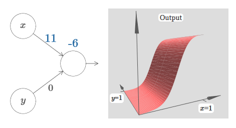
We have inputs x and y, with corresponding weights w 1 and w 2 and offset b of the neuron. Set the weight of w 2 to 0 and play with the first one, w 1 , and offset b to see how they affect the output of the neuron:
As you can see, with w 2 = 0, the input y does not affect the output of the neuron. Everything happens as if x is the only input.
Given this, what do you think will happen when we increase the weight of w 1 to w 1 = 100 and w 2 leave 0? If this is not immediately clear to you, think a little about this issue. Then watch the following video, which shows what will happen:
As before, with an increase in the input weight, the output approaches the shape of the step. The difference is that our step function is now located in three dimensions. As before, we can move the location of the steps by changing the offset. The angle will be at the point s x ≡ − b / w1.
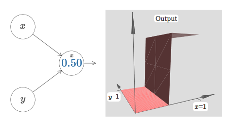
Let's redo the diagram so that the parameter is the location of the step:
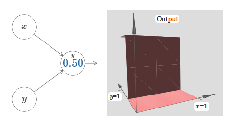
We assume that the input weight of x is of great importance - I used w 1 = 1000 - and the weight of w 2 = 0. The number on the neuron is the position of the step, and the x above it reminds us that we move the step along the x axis. Naturally, it is quite possible to obtain a step function along the y axis, making the incoming weight for y large (say, w 2 = 1000), and the weight for x equal to 0, w 1 = 0:
The number on the neuron, again, indicates the position of the step, and the y above it reminds us that we move the step along the y axis. I could directly designate the weights for x and y, but I didn’t, because that would litter the chart. But keep in mind that the y marker indicates that the weight for y is large and for x is 0.
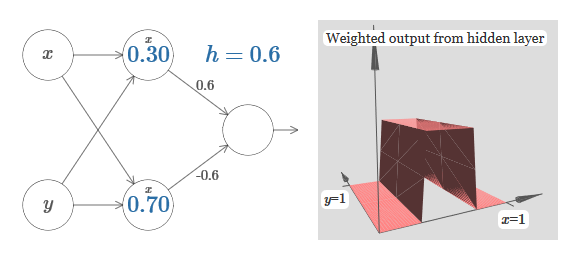
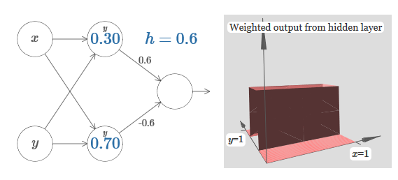
We can use the step functions we have just designed to calculate the three-dimensional protrusion function. To do this, we take two neurons, each of which will calculate a step function along the x axis. Then we combine these step functions with weights h and –h, where h is the desired height of the protrusion.All this can be seen in the following diagram:
Try changing the value of h. See how it relates to network weights. And how she changes the height of the protrusion function on the right.
Also try to change the point of the step, the value of which is set to 0.30 in the upper hidden neuron. See how it changes the shape of the protrusion. What happens if we move it beyond the 0.70 point associated with the lower hidden neuron?
We learned how to build the protrusion function along the x axis. Naturally, we can easily make the protrusion function along the y axis, using two step functions along the y axis. Recall that we can do this by making large weights at input y and setting weight 0 at input x. And so, what happens:
It looks almost identical to the previous network! The only visible change is small y markers on hidden neurons. They remind us that they produce step functions for y, and not for x, so at the input y the weight is very large and at the input x it is zero, and not vice versa. As before, I decided not to show it directly, so as not to clutter up the picture.
Let's see what happens if we add two protrusion functions, one along the x axis, the other along the y axis, both of height h:
To simplify the connection diagram with zero weight, I omitted. So far, I have left small x and y markers on hidden neurons to recall in which directions the protrusion functions are computed. Later we will refuse them, since they are implied by the incoming variable.
Try changing the parameter h. As you can see, because of this, the output weights change, as well as the weights of both protrusion functions, x and y.
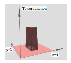
What we created is a bit like a “tower function”:
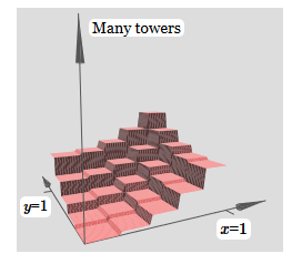
If we can create such tower functions, we can use them to approximate arbitrary functions by simply adding towers of different heights in different places:
Of course, we have not yet reached the creation of an arbitrary tower function. So far we have constructed something like a central tower of height 2h with a plateau of height h surrounding it.
But we can make a tower function. Recall that we previously showed how neurons can be used to implement the if-then-else statement:
if >= : 1 else: 0 It was a one-input neuron. And we need to apply a similar idea to the combined output of hidden neurons:
if >= : 1 else: 0 If we choose the right threshold - for example, 3h / 2, squeezed between the height of the plateau and the height of the central tower - we can crush the plateau to zero, and leave only one tower.
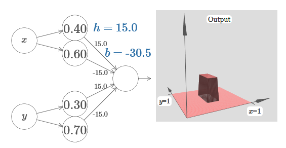
Imagine how to do this? Try experimenting with the following network. Now we are plotting the output of the entire network, and not just the weighted output of the hidden layer. This means that we add the offset term to the weighted output from the hidden layer, and apply the sigmoid. Can you find the values for h and b for which you get a tower? If you get stuck at this point, here are two tips: (1) for the outgoing neuron to show the correct behavior in the if-then-else style, we need the incoming weights (all h or –h) to be large; (2) the value of b determines the scale of the if-then-else threshold.
With default parameters, the output is similar to a flattened version of the previous diagram, with a tower and plateau. To get the desired behavior, you need to increase the value of h. This will give us threshold if-then-else behavior. Secondly, in order to set the threshold correctly, one must choose b ≈ −3h / 2.
Here's what it looks like for h = 10:
Even for relatively modest values of h, we get a nice tower function. And, of course, we can get an arbitrarily beautiful result by increasing h further and keeping the displacement at the level b = −3h / 2.
Let's try to glue two networks together to count two different tower functions. To make the respective roles of the two subnets clear, I put them in separate rectangles: each of them calculates the tower function using the technique described above. The graph on the right shows the weighted output of the second hidden layer, that is, the weighted combination of tower functions.
In particular, it can be seen that by changing the weights in the last layer, you can change the height of the output towers.
The same idea allows you to calculate as many towers as you like. We can make them arbitrarily thin and tall. As a result, we guarantee that the weighted output of the second hidden layer approximates any desired function of two variables:
In particular, by making the weighted output of the second hidden layer approximate σ −1 ⋅f well, we guarantee that the output of our network will be a good approximation of the desired function f.
What about the functions of many variables?
Let's try to take three variables, x 1 , x 2 , x 3 . Can the following network be used to calculate the tower function in four dimensions?
Here x 1 , x 2 , x 3 denote the network input. s 1 , t 1, and so on - step points for neurons - that is, all the weights in the first layer are large, and the offsets are assigned so that the points of the steps are s 1 , t 1 , s 2 , ... The weights in the second layer alternate, + h, −h, where h is some very large number. The output offset is −5h / 2.
The network computes a function equal to 1 under three conditions: x 1 is between s 1 and t 1 ; x 2 is between s 2 and t 2 ; x 3 is between s 3 and t 3 . The network is 0 in all other places. This is such a tower, in which 1 is a small portion of the entrance space, and 0 is everything else.
Gluing a lot of such networks, we can get as many towers as we like, and approximate an arbitrary function of three variables. The same idea works in m dimensions. Only the output offset (−m + 1/2) h is changed to properly squeeze the desired values and remove the plateau.
Well, now we know how to use NS to approximate the real function of many variables. What about vector functions f (x 1 , ..., x m ) ∈ R n ? Of course, such a function can be considered simply as n separate real functions f1 (x 1 , ..., x m ), f2 (x 1 , ..., x m ), and so on. And then we just glue all the networks together. So it's easy to figure it out.
Task
- We saw how to use neural networks with two hidden layers to approximate an arbitrary function. Can you prove that this is possible with one hidden layer? Hint - try working with only two output variables, and show that: (a) it is possible to get the functions of the steps not only along the x or y axes, but also in an arbitrary direction; (b) adding up many constructions from step (a), it is possible to approximate the function of a round rather than a rectangular tower; © using round towers, it is possible to approximate an arbitrary function. Step © will be easier to do using the material presented in this chapter a little below.
Going beyond sigmoid neurons
We have proven that a network of sigmoid neurons can calculate any function. Recall that in a sigmoid neuron, the inputs x 1 , x 2 , ... turn at the output into σ (∑ j w j x j j + b), where w j are the weights, b is the bias, and σ is the sigmoid.
What if we look at another type of neuron using a different activation function, s (z):
That is, we will assume that if a neuron has x 1 , x 2 , ... weights w 1 , w 2 , ... and bias b, then s (∑ j w j x j + b) will be output.
We can use this activation function to get stepped, just like in the case of the sigmoid. Try (in the original article ) on the diagram to lift up the weight to, say, w = 100:
As in the case of the sigmoid, because of this, the activation function is compressed, and as a result turns into a very good approximation of the step function. Try changing the offset, and you will see that we can change the location of the step to any. Therefore, we can use all the same tricks as before to calculate any desired function.
What properties should s (z) have in order for this to work? We need to assume that s (z) is well defined as z → −∞ and z → ∞. These limits are two values accepted by our step function. We also need to assume that these limits are different. If they didn’t differ, the steps would not work; there would simply be a flat schedule! But if the activation function s (z) satisfies these properties, the neurons based on it are universally suitable for calculations.
Tasks
- Earlier in the book, we met a different type of neuron — a straightened linear neuron, or a rectified linear unit, [ReLU]. Explain why such neurons do not satisfy the conditions necessary for universality. Find evidence of versatility showing that ReLUs are universally suitable for computing.
- Suppose we consider linear neurons with an activation function s (z) = z. Explain why linear neurons do not satisfy the conditions of universality. Show that such neurons cannot be used for universal computing.
Fix step function
For the time being, we assumed that our neurons produce accurate step functions. This is a good approximation, but only an approximation. In fact, there is a narrow gap of failure, shown in the following graph, where the functions do not behave at all like a step function:
In this period of failure, my explanation of universality does not work.
Failure is not so scary. By setting sufficiently large input weights, we can make these gaps arbitrarily small. We can make them much smaller than on the chart, invisible to the eye. So maybe we don’t have to worry about this problem.
Nevertheless, I would like to have some way to solve it.
It turns out that it’s easy to solve. Let’s look at this solution for calculating NS functions with only one input and output. The same ideas will work to solve the problem with a large number of inputs and outputs.
In particular, let's say we want our network to compute some function f. As before, we try to do this by designing the network so that the weighted output of the hidden layer of neurons is σ −1 ⋅f (x):
If we do this using the technique described above, we will make the hidden neurons give out a sequence of functions of the protrusions:
Of course, I exaggerated the size of the intervals of failure, so that they were easier to see. It should be clear that if we add up all these functions of the protrusions, we get a fairly good approximation of σ −1 ⋅f (x) everywhere except for the intervals of failure.
But, suppose that instead of using the approximation just described, we use a set of hidden neurons to calculate the approximation of half of our original objective function, i.e., σ −1 ⋅f (x) / 2. Of course, it will look just like a scaled version of the latest graph:
And suppose we make one more set of hidden neurons calculate the approximation to σ −1 ⋅f (x) / 2, however, at its base the protrusions will be shifted by half their width:
Now we have two different approximations for σ − 1⋅f (x) / 2. If we add up these two approximations, we obtain a general approximation to σ − 1⋅f (x). This general approximation will still have inaccuracies in small intervals. But the problem will be less than before - because the points falling into the intervals of the failure of the first approximation will not fall into the intervals of the failure of the second approximation. Therefore, the approximation in these intervals will be approximately 2 times better.
We can improve the situation by adding a large number, M, of overlapping approximations of the function σ − 1⋅f (x) / M. If all of their failure intervals are narrow enough, any current will be in only one of them. If you use a sufficiently large number of overlapping approximations of M, the result will be an excellent general approximation.
Conclusion
The explanation of universality discussed here definitely cannot be called a practical description of how to count functions using neural networks! In this sense, it is more like proof of the versatility of NAND logic gates and more. Therefore, I basically tried to make this design clear and easy to follow without optimizing its details. However, trying to optimize this design can be an interesting and instructive exercise for you.
Although the result obtained cannot be directly used to create NS, it is important because it removes the question of the computability of any particular function using NS. The answer to such a question will always be positive. Therefore, it is correct to ask if any function is computable, but what is the correct way to calculate it.
Our universal design uses only two hidden layers to calculate an arbitrary function. As we discussed, it is possible to get the same result with a single hidden layer. Given this, you may wonder why we need deep networks, that is, networks with a large number of hidden layers. Can't we just replace these networks with shallow ones that have one hidden layer?
Although, in principle, it is possible, there are good practical reasons for using deep neural networks. As described in Chapter 1, deep NSs have a hierarchical structure that allows them to adapt well to study hierarchical knowledge, which are useful for solving real problems. More specifically, when solving problems such as pattern recognition, it is useful to use a system that understands not only individual pixels, but also increasingly complex concepts: from borders to simple geometric shapes, and beyond, to complex scenes involving several objects. In later chapters we will see evidence in favor of the fact that deep NSs will be better able to cope with the study of such hierarchies of knowledge than shallow ones. To summarize: universality tells us that NS can calculate any function; empirical evidence suggests that deep NSs are better adapted to the study of functions useful for solving many real-world problems.
Source: https://habr.com/ru/post/461659/
All Articles