Brief article on business process mining in the context of growing interest in the concept of "digital twin". Due to the periodic emergence of this topic, I consider it appropriate to share approaches to the solution.

Formulation of the problem

The situation is extremely simple.

• There is company X (Y, Z, ...).
• The company has business processes automated by various IT systems.
• There are business analysts who have drawn bpmn diagrams for these processes. More specifically, their own "bpmn idea" of how these processes should have looked.
• Business users want some kind of presentation (KPI) on these processes.

How to get to the truth and count these metrics?

It is a continuation of previous publications .

We formulate the task in a computer-friendly manner.

Basic postulates:

• There is a temporary event log (various logs of IT systems, cdr \ xdr, just records of events in the database) of varying degrees of purity, completeness and consistency.
• IT systems act as a state machine and “walk” between different states in accordance with the actions of users and the business logic laid down by the programmers in them.
• User interaction is carried out in a transactional form.

Physical world corrections:

• The number of changes made to IT systems is such that bpmn diagrams of business analysts have almost nothing to do with reality.
• Data can be very unstructured (for example, application logs).
• "Transactional" is a logical concept. The event records themselves contain only attributes inherent in this state and there is no end-to-end transaction identifier.
• The number of records per day is tens, hundreds, thousands of millions of pieces .

Set-Count Solution

To solve such problems it is necessary:

• Reconstruct transactions
• Reconstruct real business processes
• make calculations;
• generate results in human-readable format.

You can start looking for vendor solutions and pay millions. But we have R. in our hands. It perfectly allows us to solve this problem. Brief considerations below.

Everything seems simple and R has a good consistent set of bupaR packages. But a fly in the ointment is present and it poisons everything. This set in an acceptable time can only cope with a small number of events (hundreds of thousands - several million).
For large volumes, other approaches must be used.

Add speed!

Emulate an input dataset

To demonstrate ideas, it is necessary to form some kind of test data set. Let’s take an example of a federal chain of stores as a physical source for a mathematical model. Fortunately, this is understandable to everyone. Although with the same success it can be ATMs, call centers, public transport, water supply, etc.

• There are shops of various sizes (small, medium and large).
• In stores there are cash desks (pos terminals).
• Store numbers can be alphanumeric; terminal numbers can be digital.
• Shoppers go to the stores and make purchases of something while paying with a card.
• The interaction of the pos terminal with the card and the bank is described by a certain set of states and the rules for the transition between them.
• Transactions are successful, unsuccessful, deferred and incomplete (the bank is unavailable, for example).
• Transactions have timeouts.

Take the following set of business transaction patterns:

"INIT-REQUEST-RESPONSE-SUCCESS" "INIT-REQUEST-RESPONSE-ERROR" "INIT-REQUEST-RESPONSE-DEFFERED" "INIT-REQUEST" "INIT" 

To demonstrate the approach, we will create a small sample, but it all works fine on billions of records (for such a volume without superdeep optimization, the characteristic time is measured in only hundreds of seconds on a single server of very mediocre performance).

Direct spoilers for large volumes:

• in many places, tidyverse means tidyverse can’t get an answer;
• optimizing even microsteps is useful and can make a significant contribution.

 library(tidyverse) library(datapasta) library(tictoc) library(data.table) library(stringi) library(anytime) library(rTRNG) data.table::setDTthreads(0) #      data.table data.table::getDTthreads() #     set.seed(46572) RcppParallel::setThreadOptions(numThreads = parallel::detectCores() - 1) #   --   -,     #  5   -, 2  --   bo_pattern <- tibble::tribble( #  ,    ,    ~pattern, ~prob, ~mean_duration, "INIT-REQUEST-RESPONSE-SUCCESS", 0.7, 5, "INIT-REQUEST-RESPONSE-ERROR", 0.15, 5, "INIT-REQUEST-RESPONSE-DEFFERED", 0.07, 8, "INIT-REQUEST", 0.05, 2, "INIT", 0.03, 0.5 ) #    +     checkmate::assertTRUE(sum(bo_pattern$prob) == 1) df <- bo_pattern %>% separate_rows(pattern) %>% #   mutate(coeff = sum(prob)) %>% group_by(pattern) %>% #    summarise(event_prob = sum(prob/coeff)*100) %>% ungroup() checkmate::assertTRUE(sum(df$event_prob) == 100) #   3  :  (4 ),  (12 ),  (30 ) df1 <- tribble( ~type, ~n_pos, ~n_store, "small", 4, 10, "medium", 12, 5, "large", 30, 2 ) %>% #       mutate(store = map2(row_number(), n_store, ~sample(x = .x * 1000 + 1:.y, size = .y, replace = FALSE))) %>% unnest(store) %>% #       mutate(pos = map(n_pos, ~sample(x = .x, size = .x, replace = FALSE))) %>% unnest(pos) %>% mutate(pattern = sample(bo_pattern$pattern, n(), replace = TRUE, prob = bo_pattern$prob)) tic("Generate transactions") #     ,      #         ,       df2 <- df1 %>% #         select(-matches("duration")) %>% left_join(bo_pattern, by = "pattern") %>% #   sample_frac(size = 200, replace = TRUE) %>% mutate(duration = rnorm(n(), mean = mean_duration, sd = mean_duration * .25)) %>% select(-prob, -mean_duration) %>% #   ,      >  #    30  filter(duration > 0.5 & duration < 30) %>% #    POS       mutate(session_id = row_number()) %>% #     ,       separate_rows(pattern) %>% rename(event = pattern) toc() tic("Generate time markers, data.table way") samples_tbl <- data.table::as.data.table(df2) %>% # setkey(session_id, duration, physical = FALSE) %>% #           # 1-       , ,      5  # .[, ticks := base::sort(runif(.N, 5, 5 + duration)), by = .(session_id, duration)] %>% #          match.arg   base::order!! #     #       0  1     #     # .[, tshift := runif(.N, 0, 1)] %>% #    trng     (    ) # ,           .[, trand := runif_trng(.N, 0, 1, parallelGrain = 100L) * duration] %>% #      ,      # .[, ticks := sort(tshift), by = .(session_id)] %>% #  ,     session_id,   ,     .[, t_idx := session_id + trand / max(trand)/10] %>% #         # session_id            .  .[, tshift := (sort(t_idx) - session_id) * 10 * max(trand)] %>% #   ,     POS     (60 ) .[event == "INIT", tshift := tshift + runif_trng(.N, 0, 60, parallelGrain = 100L)] %>% #     .[, `:=`(duration = NULL, trand = NULL, t_idx = NULL, n_store = NULL, n_pos = NULL, timestamp = as.numeric(anytime("2019-03-11 08:00:00 MSK")))] %>% #     ,   01.03.2019     .[, timestamp := timestamp + cumsum(tshift), by = .(store, pos)] %>% #      .[timestamp <= as.numeric(anytime("2019-04-11 23:00:00 MSK")), ] %>% #           .[, timestamp := anytime(timestamp, tz = "Europe/Moscow")] %>% as_tibble() %>% select(store, pos, event, timestamp, session_id) toc() 

For the purity of the experiment, we leave only the significant parameters and mix everything. In real life, it is still necessary to randomly throw out part of the fragments (possibly in separate time blocks), thereby emulating losses in receiving data.

 #   log_tbl <- samples_tbl %>% select(store, pos, state = event, timestamp_msk = timestamp) %>% sample_n(n()) #   log_tbl %>% mutate(timegroup = lubridate::ceiling_date(timestamp_msk, unit = "10 mins")) %>% ggplot(aes(timegroup)) + # geom_bar(width = 0.7*600) + geom_bar(colour = "white", size = 1.3) + theme_bw()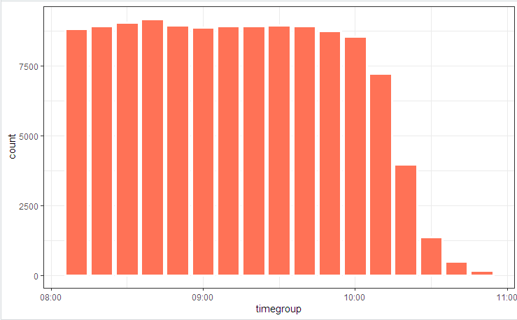 

We illustrate the process diagram with a picture

and state distribution

Slight fluctuations are due to the fact that the table is considered at the beginning (it is included in the code), and bupaR::process_map worked at the end when some of the randomly generated data that did not fit the integral constraints was cut off by filtering elements.

Transaction Reconstruction

The first thing that is usually offered when you have to collect / disassemble / compare time series is groupings and comparison cycles. In demos with 100 entries, this hike will work, but millions of lists will not. To cope with this task, you need to localize the time loss points (internal loops, intermediate memory allocations and copying) and try to eliminate them to a minimum.

As a result, this problem can be reduced to ten lines.

 clean_dt <- as.data.table(log_tbl) %>% #     INIT .[, start := (state == "INIT")] %>% #  session_id      ,  #             .[, event_date := lubridate::as_date(timestamp_msk)] %>% .[, date_str := format(.BY[[1]], "%y%m%d"), by = event_date] %>% #            # timestamp_msk    setorder(store, pos, timestamp_msk) %>% #     --              .[, session_id := paste(date_str, store, pos, cumsum(start), sep = "_")] %>% #        ( 30 ) # .[, time_shift := timestamp_msk - shift(timestamp_msk), by = .(store, pos)] %>% #        ,   INIT .[, time_locf := cummax(as.numeric(timestamp_msk) * as.numeric(start)), by = .(store, pos)] %>% .[, time_shift := as.numeric(timestamp_msk) - time_locf] %>% #   ,       30  .[, lost_chain := time_shift > 30] %>% # .[, time_shift := as.numeric(!start) * as.numeric(timestamp_msk - shift(timestamp_msk, fill = 0))] %>% # INIT    # .[, time_accu := cumsum(time_shift)] %>% .[, date_str := NULL] #          #    tidyverse  ,      dt <- as.data.table(clean_dt) %>% #     !!! .[lost_chain != TRUE] %>% #        1-    .[order(timestamp_msk, store, pos)] %>% .[, bp_pattern := stri_join(state, collapse = "-"), by = session_id] #     as_tibble(dt) %>% distinct(session_id, bp_pattern) %>% count(session_id, sort = TRUE) 

In a few seconds, we have a reconstructed picture of business processes.

And (who would have thought !!!) in fact, it turns out that business processes automated in IT systems work somewhat differently (or not at all) as business analysts convinced everyone. The wonders and arguments of the “process owners” will accompany the study of the final picture.

Actively apply tricks

When computing speed becomes an important quantity, writing a working code is not enough. It is necessary to pay attention to all levels. There are also a number of algorithmic tricks that can significantly reduce the execution time.

In particular, the following can be mentioned in this task:

1. For the main processing, only data.table (speed, work on links), + accounting for internal query optimization.
2. POSIXct can contain milliseconds (although it doesn’t display normally, but can be corrected using options(digits.secs=X) ), we hide them there, it will be easier to compare and sort.
3. Avoid physical sorting within groups! .. A single physical sorting of the entire vector ensures that the data is sorted in groups.
4. Avoid computing within groups. We try to do all that is possible on the source data (we apply vectorization, reduce the invoices for function calls).
5. We use a transaction timeout to deal with time gaps.
6. The locf (Last Observation Carried Forward) methods are slow. To transfer properties on a timeline, use cumsum , cummax .
7. Time-consuming operations, such as POSIX -> string conversion, regular search, etc. We do not do it element by element, but on convolutions. Overheads for internal indexing and grouping of the converted field are incomparably smaller.
8. We actively use multithreading (including intra-packet).
9. Do not neglect microoptimization. For example, stri_c is several times faster than paste0 .

 #  1 log <- getLog(fileName) bench::mark( paste0 = paste0(log$value, collapse = "\n"), stringi = stri_c(log$value, collapse = "\n") ) # # A tibble: 2 x 13 # expression min median `itr/sec` mem_alloc `gc/sec` n_itr n_gc total_time # <bch:expr> <bch:> <bch:> <dbl> <bch:byt> <dbl> <int> <dbl> <bch:tm> # 1 paste0 58ms 59.1ms 16.9 496KB 0 9 0 533ms # 2 stringi 16.9ms 17.5ms 57.1 0B 0 29 0 508ms 

Previous post - Swiss knife for processing json .