Emotion recognition using a convolutional neural network

Recognizing emotions has always been an exciting challenge for scientists. Recently, I have been working on an experimental SER project (Speech Emotion Recognition) to understand the potential of this technology - for this I selected the most popular repositories on Github and made them the basis of my project.

Before we begin to understand the project, it will be nice to remember what kind of bottlenecks SER has.

Main obstacles

• emotions are subjective, even people interpret them differently. It is difficult to define the very concept of “emotion”;
• commenting on audio is hard. Should we somehow mark every single word, sentence, or the entire communication as a whole? A set of what kind of emotions to use in recognition?
• collecting data is also not easy. A lot of audio data can be collected from movies and news. However, both sources are “biased” because the news must be neutral, and the emotions of the actors are played. It is difficult to find an “objective” source of audio data.
• markup data requires large human and time resources. Unlike drawing frames on images, it requires specially trained personnel to listen to entire audio recordings, analyze them and provide comments. And then these comments must be appreciated by many other people, because the ratings are subjective.

Project Description

Using a convolutional neural network to recognize emotions in audio recordings. And yes, the owner of the repository did not refer to any sources.

Data Description

There are two datasets that were used in the RAVDESS and SAVEE repositories, I just adapted RAVDESS in my model. There are two types of data in the RAVDESS context: speech and song.
')
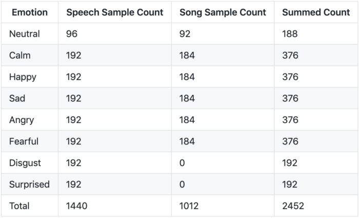
Dataset RAVDESS (The Ryerson Audio-Visual Database of Emotional Speech and Song) :

• 12 actors and 12 actresses recorded their speech and songs in their performance;
• actor # 18 has no recorded songs;
• emotions Disgust (aversion), Neutral (neutral) and Surprises (surprise) are absent in the "song" data.

Emotion Breakdown:


Emotion Distribution Chart:

Feature extraction

When we work with speech recognition tasks, the cepstral coefficient (MFCCs) is an advanced technology, despite the fact that it appeared in the 80s.

Quote from the MFCC Tutorial :

This shape determines what the output sound is. If we can pinpoint the form, it will give us an accurate representation of the phoneme sounded. The shape of the vocal tract manifests itself in an envelope of a short spectrum, and the MFCC works to accurately display this envelope.

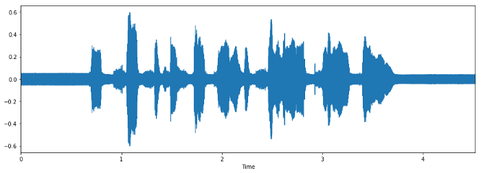
Waveform


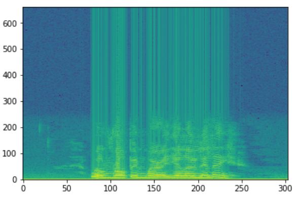
Spectrogram

We use MFCC as an input feature. If you are interested in learning more about what MFCC is, then this tutorial is for you. Downloading data and converting it to the MFCC format can be easily done using the librosa Python package.

Default Model Architecture

The author developed a CNN model using the Keras package, creating 7 layers - six Con1D layers and one density layer (Dense).

model = Sequential() model.add(Conv1D(256, 5,padding='same', input_shape=(216,1))) #1 model.add(Activation('relu')) model.add(Conv1D(128, 5,padding='same')) #2 model.add(Activation('relu')) model.add(Dropout(0.1)) model.add(MaxPooling1D(pool_size=(8))) model.add(Conv1D(128, 5,padding='same')) #3 model.add(Activation('relu')) #model.add(Conv1D(128, 5,padding='same')) #4 #model.add(Activation('relu')) #model.add(Conv1D(128, 5,padding='same')) #5 #model.add(Activation('relu')) #model.add(Dropout(0.2)) model.add(Conv1D(128, 5,padding='same')) #6 model.add(Activation('relu')) model.add(Flatten()) model.add(Dense(10)) #7 model.add(Activation('softmax')) opt = keras.optimizers.rmsprop(lr=0.00001, decay=1e-6) 

The author commented on layers 4 and 5 in the latest release (September 18, 2018) and the final file size of this model does not fit the network provided, so I can not achieve the same result in accuracy - 72%.

The model is simply trained with the parameters batch_size=16 and epochs=700 , without any training schedule, etc.

 # Compile Model model.compile(loss='categorical_crossentropy', optimizer=opt,metrics=['accuracy']) # Fit Model cnnhistory=model.fit(x_traincnn, y_train, batch_size=16, epochs=700, validation_data=(x_testcnn, y_test)) 

Here categorical_crossentropy is a function of losses, and the measure of evaluation is accuracy.

My experiment

Exploratory data analysis

In the RAVDESS dataset, each actor shows 8 emotions, pronouncing and singing 2 sentences, 2 times each. As a result, 4 examples of each emotion are obtained from each actor, with the exception of the above-mentioned neutral emotions, disgust, and surprise. Each audio lasts approximately 4 seconds, in the first and last seconds most often silence.

Typical offers :

Observation

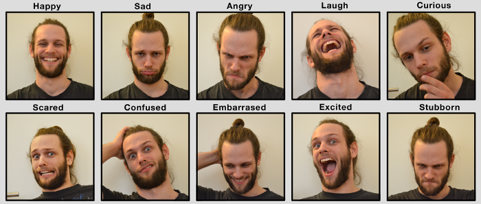
After I selected a dataset from 1 actor and 1 actress, and then listened to all their records, I realized that men and women express their emotions in different ways. For example:

• male anger (Angry) is just louder;
• men's joy (Happy) and frustration (Sad) - a feature in laughing and crying tones during the "silence";
• female joy (Happy), anger (Angry) and frustration (Sad) are louder;
• female disgust (Disgust) contains the sound of vomiting.

Experiment repetition

The author removed the neutral, disgust, and surprised classes to make the 10-class recognition of the RAVDESS dataset. Trying to repeat the author’s experience, I got the following result:



However, I found out that there is a data leak when the dataset for validation is identical to the test dataset. Therefore, I repeated the separation of the data, isolating the datasets of two actors and two actresses so that they were not visible during the test:

• actors 1 to 20 are used for Train / Valid sets in an 8: 2 ratio;
• actors 21 to 24 are isolated from the tests;
• Train Set parameters: (1248, 216, 1);
• Valid Set parameters: (312, 216, 1);
• Test Set parameters: (320, 216, 1) - (isolated).

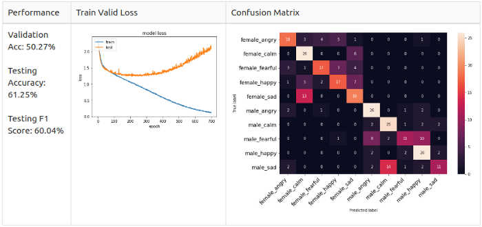
I re-trained the model and here is the result:

Performance test

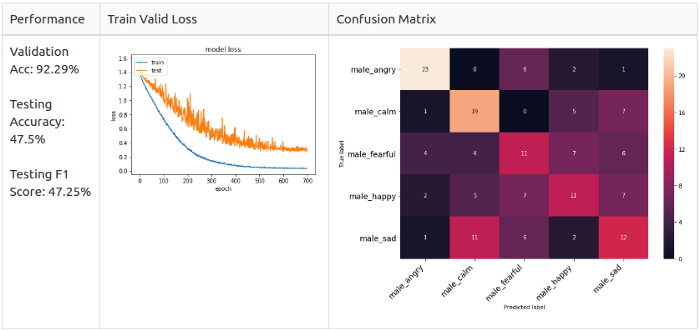
From the Train Valid Gross graph it is clear that there is no convergence for the selected 10 classes. Therefore, I decided to reduce the complexity of the model and leave only male emotions. I isolated two actors in the test set, and put the rest in the train / valid set, 8: 2 ratio. This ensures that there is no imbalance in the dataset. Then I coached the male and female data separately to conduct the test.

Male dataset

• Train Set - 640 samples from actors 1-10;
• Valid Set - 160 samples from actors 1-10;
• Test Set - 160 samples from actors 11-12.

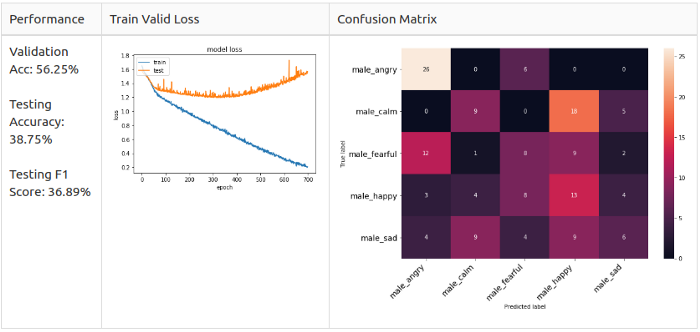
Reference line: men


Female dataset

• Train Set - 608 samples from actresses 1-10;
• Valid Set - 152 samples from actresses 1-10;
• Test Set - 160 samples from actresses 11-12.

Reference line: women


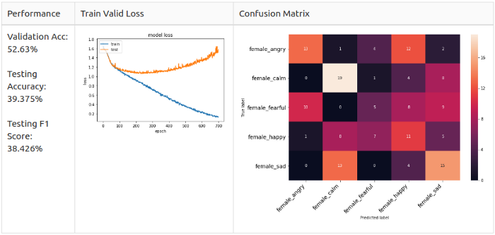
As you can see, error matrices are different.

Men: Angry and Happy are the main predicted classes in the model, but they are not alike.

Women: disorder (Sad) and joy (Happy) - basically predicted classes in the model; anger and joy are easily confused.

Recalling the observations from the Intelligence Data Analysis , I suspect that female Angry and Happy are similar to the point of confusion because their way of expression is simply to increase their voices.

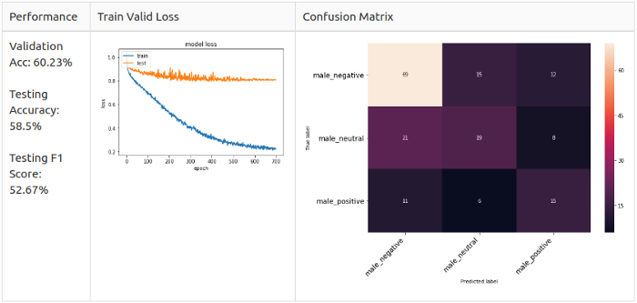
On top of that, I'm curious that if I simplify the model even further, leave only the Positive, Neutral, and Negative classes. Or only Positive and Negative. In short, I grouped emotions into 2 and 3 classes, respectively.

2 classes:

• Positive: joy (Happy), calm (Calm);
• Negative: angry, fearful, frustration (sad).

3 classes:

• Positive: joy (Happy);
• Neutral: calm (Calm), neutral (Neutral);
• Negative: angry, fearful, frustration (sad).

Before starting the experiment, I set up the model architecture using male data, making 5-class recognition.

 #   -  target_class = 5 #  model = Sequential() model.add(Conv1D(256, 8, padding='same',input_shape=(X_train.shape[1],1))) #1 model.add(Activation('relu')) model.add(Conv1D(256, 8, padding='same')) #2 model.add(BatchNormalization()) model.add(Activation('relu')) model.add(Dropout(0.25)) model.add(MaxPooling1D(pool_size=(8))) model.add(Conv1D(128, 8, padding='same')) #3 model.add(Activation('relu')) model.add(Conv1D(128, 8, padding='same')) #4 model.add(Activation('relu')) model.add(Conv1D(128, 8, padding='same')) #5 model.add(Activation('relu')) model.add(Conv1D(128, 8, padding='same')) #6 model.add(BatchNormalization()) model.add(Activation('relu')) model.add(Dropout(0.25)) model.add(MaxPooling1D(pool_size=(8))) model.add(Conv1D(64, 8, padding='same')) #7 model.add(Activation('relu')) model.add(Conv1D(64, 8, padding='same')) #8 model.add(Activation('relu')) model.add(Flatten()) model.add(Dense(target_class)) #9 model.add(Activation('softmax')) opt = keras.optimizers.SGD(lr=0.0001, momentum=0.0, decay=0.0, nesterov=False) 

I added 2 layers of Conv1D, one layer of MaxPooling1D and 2 layers of BarchNormalization; I also changed the dropout value to 0.25. Finally, I changed the optimizer to SGD with a learning speed of 0.0001.

 lr_reduce = ReduceLROnPlateau(monitor='val_loss', factor=0.9, patience=20, min_lr=0.000001) mcp_save = ModelCheckpoint('model/baseline_2class_np.h5', save_best_only=True, monitor='val_loss', mode='min') cnnhistory=model.fit(x_traincnn, y_train, batch_size=16, epochs=700, validation_data=(x_testcnn, y_test), callbacks=[mcp_save, lr_reduce]) 

To train the model, I applied a reduction in the “training plateau” and saved only the best model with a minimum value of val_loss . And here are the results for the different target classes.

New model performance

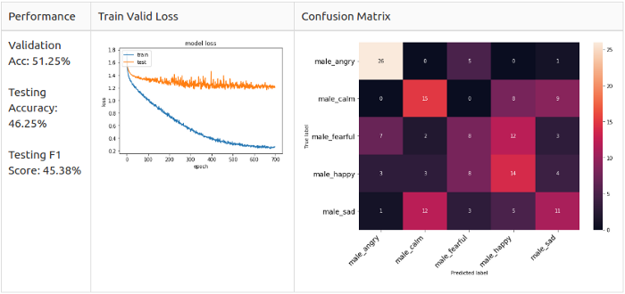
Men, 5 classes



Women, Grade 5

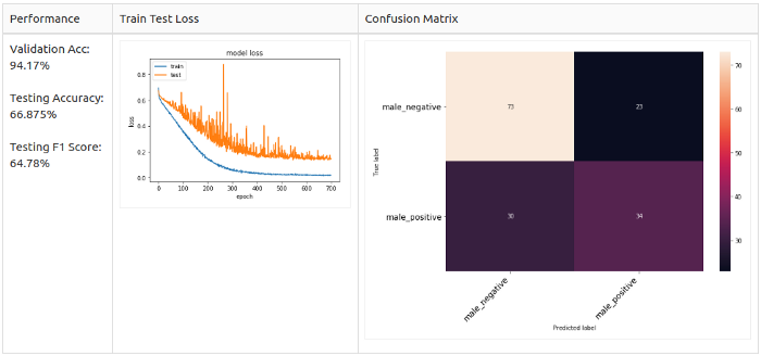
Men, Grade 2


Men, Grade 3

Increase (augmentation)

When I strengthened the architecture of the model, the optimizer and the speed of training, it turned out that the model still does not converge in training mode. I suggested that this is a data quantity problem, since we only have 800 samples. This led me to methods of increasing audio, in the end I doubled the datasets. Let's take a look at these methods.

Men, Grade 5

Dynamic Increment

 def dyn_change(data): """    """ dyn_change = np.random.uniform(low=1.5,high=3) return (data * dyn_change) 

Pitch Adjustment

 def pitch(data, sample_rate): """    """ bins_per_octave = 12 pitch_pm = 2 pitch_change = pitch_pm * 2*(np.random.uniform()) data = librosa.effects.pitch_shift(data.astype('float64'), sample_rate, n_steps=pitch_change, bins_per_octave=bins_per_octave)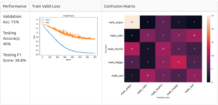 

Bias

 def shift(data): """   """ s_range = int(np.random.uniform(low=-5, high = 5)*500) return np.roll(data, s_range)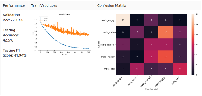 

Adding White Noise

 def noise(data): """    """ #     : https://docs.scipy.org/doc/numpy-1.13.0/reference/routines.random.html noise_amp = 0.005*np.random.uniform()*np.amax(data) data = data.astype('float64') + noise_amp * np.random.normal(size=data.shape[0]) return data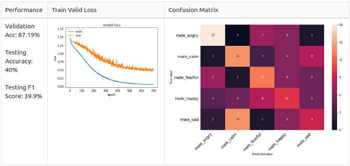 

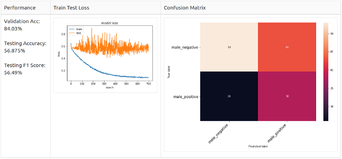
It is noticeable that augmentation greatly increases accuracy, up to 70 +% in the general case. Especially in the case of the addition of white, which increases the accuracy to 87.19% - however, the test accuracy and the F1 measure fall by more than 5%. And then I got the idea to combine several augmentation methods for a better result.

Combining several methods

White noise + bias

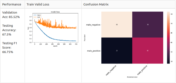
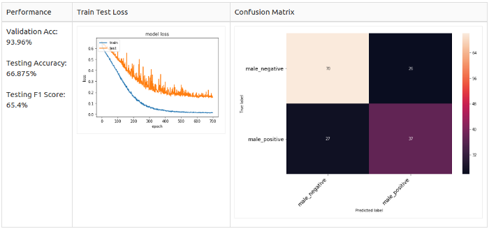
Testing augmentation on men

Men, Grade 2

White noise + bias

For all samples


White noise + bias

Only for positive samples, since the 2-class set is unbalanced (towards negative samples).


Pitch + White Noise
For all samples


Pitch + White Noise

For positive samples only

Conclusion

In the end, I was able to experiment only with a male dataset. I re-divided the data so as to avoid imbalance and, as a consequence, data leakage. I set up the model to experiment with male voices, as I wanted to simplify the model as much as possible to get started. I also conducted tests using different augmentation methods; the addition of white noise and bias have worked well on unbalanced data.

findings

• emotions are subjective and difficult to fix;
• it is necessary to determine in advance which emotions are suitable for the project;
• Do not always trust content with Github, even if it has many stars;
• data sharing - keep it in mind;
• exploratory data analysis always gives a good idea, but you need to be patient when it comes to working with audio data;
• Determine what you will give to the input of your model: a sentence, an entire record or an exclamation?
• lack of data is an important success factor in SER, however, creating a good dataset with emotions is a complex and expensive task;
• simplify your model in case of lack of data.

Further improvement

• I used only the first 3 seconds as input to reduce the overall size of the data - the original project used 2.5 seconds. I would like to experiment with full-sized recordings;
• you can pre-process the data: trim the silence, normalize the length by padding with zeros, etc .;
• try recurrent neural networks for this task.