New GPU Tracking Algorithm: Wavefront Path Tracing

In this article, we explore the important concept used in the recently released Lighthouse 2 platform. Wavefront path tracing , as it is called Lane, Karras and Aila from NVIDIA, or streaming path tracing, as it was originally called in Van Antwerp ’s master's thesis , plays a crucial role in developing efficient path tracers on the GPU, and potentially path tracers on the CPU. However, it is quite counterintuitive, therefore, to understand it, it is necessary to rethink ray tracing algorithms.

Occupancy

The path tracing algorithm is surprisingly simple and can be described in just a few lines of pseudocode:

vec3 Trace( vec3 O, vec3 D ) IntersectionData i = Scene::Intersect( O, D ) if (i == NoHit) return vec3( 0 ) // ray left the scene if (i == Light) return i.material.color // lights do not reflect vec3 R, pdf = RandomDirectionOnHemisphere( i.normal ), 1 / 2PI return Trace( i.position, R ) * i.BRDF * dot( i.normal, R ) / pdf 

The input is the primary ray passing from the camera through the screen pixel. For this beam, we determine the closest intersection with the scene primitive. If there are no intersections, then the beam disappears into the void. Otherwise, if the beam reaches the light source, then we found the light path between the source and the camera. If we find something else, then we perform reflection and recursion, hoping that the reflected beam will still find the source of illumination. Note that this process resembles the (return) path of a photon reflecting off the surface of a scene.

GPUs are designed to perform this task in multi-threaded mode. At first it might seem that ray tracing is ideal for this. So, we use OpenCL or CUDA to create a stream for a pixel, each stream performs an algorithm that actually works as intended, and is pretty fast: just look at a few examples with ShaderToy to understand how fast ray tracing can be on the GPU. But be that as it may, the question is different: are these ray tracers really as fast as possible ?
')

This algorithm has a problem. The primary ray can find the light source immediately, or after one random reflection, or after fifty reflections. The programmer for the CPU will notice a potential stack overflow here; the GPU programmer should see the occupancy problem . The problem is caused by conditional tail recursion: the path may end at the light source or continue on. Let's transfer this to many threads: some of the threads will stop, and the other part will continue to work. After a few reflections, we will have several threads that need to continue computing, and most threads will wait for these last threads to finish working. Employment is a measure of the portion of GPU threads that do useful work.

The employment problem applies to the execution model of SIMT GPU devices. Streams are organized into groups, for example, in Pascal GPU (NVidia equipment class 10xx) 32 threads are combined into a warp . Threads in warp have a common program counter: they are executed with a fixed step, so each program instruction is executed by 32 threads simultaneously. SIMT stands for single instruction multiple thread , which describes the concept well. For a SIMT processor, a code with conditions is complex. This is clearly shown in the official Volta documentation:


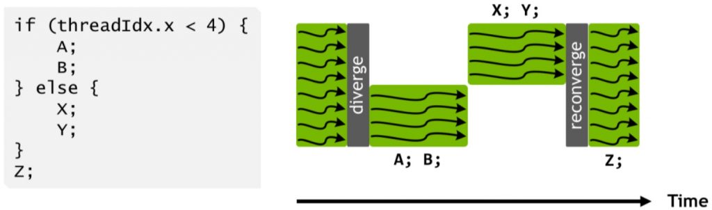
Code execution with conditions in SIMT.

When a certain condition is true for some threads in warp, the branches of the if-statement are serialized. An alternative to the “all threads do the same” approach is “some threads are disabled”. In the if-then-else block, the average occupation of warp will be 50%, unless all threads have consistency regarding the condition.

Unfortunately, code with conditions in the ray tracer is not so rare. Rays of shadows are emitted only if the light source is not behind the shading point, different paths may collide with different materials, integration with the Russian roulette method can destroy or leave the path alive, and so on. It turns out that occupancy is becoming the main source of inefficiency, and it is not so easy to prevent it without emergency measures.

Streaming Path Tracing

The streaming path tracing algorithm is designed to address the root cause of the busy problem. Streaming path tracing divides the path tracing algorithm into four steps:

1. Generate
2. Extend
3. Shade
4. Connect

Each stage is implemented as a separate program. Therefore, instead of executing a full path tracer as a single GPU program (“kernel”, kernel), we will have to work with four cores. In addition, as we will soon see, they are executed in a loop.

Stage 1 (“Generate”) is responsible for the generation of primary rays. This is a simple core that creates the starting points and directions of the rays in an amount equal to the number of pixels. The output of this stage is a large ray buffer and a counter informing the next stage of the number of rays that need to be processed. For primary rays, this value is equal to the width of the screen times the height of the screen .

Stage 2 (“Renew”) is the second core. It is executed only after stage 1 is completed for all pixels. The kernel reads the buffer generated in step 1 and crosses each ray with the scene. The output of this stage is the intersection result for each ray stored in the buffer.

Stage 3 (“Shade”) is performed after the completion of stage 2. It receives the result of the intersection from stage 2 and calculates the shading model for each path. This operation may or may not generate new rays, depending on whether the path has completed. The paths that generate the new ray (the path “extends”) writes the new ray (the “path segment”) to the buffer. Paths that directly sample light sources (“explicitly sample lighting” or “calculate the next event”) write a shadow beam to a second buffer.

Stage 4 (“Connect”) traces the shadow rays generated in stage 3. This is similar to stage 2, but with an important difference: the rays of the shadow need to find any intersection, while the extending rays need to find the nearest intersection. Therefore, a separate core has been created for this.

After completing step 4, we get a buffer containing rays that extend the path. Having taken these rays, we proceed to stage 2. We continue to do this until there are no extension rays or until we reach the maximum number of iterations.

Sources of Inefficiency

A programmer concerned about performance will see a lot of dangerous moments in such a scheme of streaming path tracing algorithms:

• Instead of a single kernel call, we now have three calls per iteration , plus a generation kernel. Challenges of the cores mean a certain increase in load, so this is bad.
• Each core reads a huge buffer and writes a huge buffer.
• The CPU needs to know how many threads to generate for each core, so the GPU should tell the CPU how many rays were generated in step 3. Moving information from the GPU to the CPU is a bad idea, and it needs to be done at least once per iteration.
• How does stage 3 write the rays to the buffer without creating spaces everywhere? He doesn’t use an atomic counter for this?
• The number of active paths is still decreasing, so how can this scheme help at all?

Let's start with the last question: if we transfer a million tasks to the GPU, it will not generate a million threads. The true number of threads executed simultaneously depends on the equipment, but in the general case, tens of thousands of threads are executed. Only when the load falls below this number will we notice employment problems caused by a small number of tasks.

Another concern is the large-scale I / O of buffers. This is indeed a difficulty, but not as serious as you might expect: data access is highly predictable, especially when writing to buffers, so the delay does not cause problems. In fact, GPUs were primarily developed for this type of data processing.

Another aspect that GPUs handle very well is atomic counters, which is quite unexpected for programmers working in the CPU world. The z-buffer requires quick access, and therefore the implementation of atomic counters in modern GPUs is extremely effective. In practice, an atomic write operation is as costly as an uncached write to global memory. In many cases, the delay will be masked by large-scale parallel execution in the GPU.

Two questions remain: kernel calls and two-way data transfer for counters. The latter is actually a problem, so we need another architectural change: persistent threads .

Effects

Before delving into the details, we will look at the implications of using the wavefront path tracing algorithm. First, let's say about buffers. We need a buffer to output the data of stage 1, i.e. primary rays. For each beam we need:

• Ray origin: three float values, i.e. 12 bytes
• Ray direction: three float values, i.e. 12 bytes

In practice, it is better to increase the size of the buffer. If you store 16 bytes for the beginning and direction of the beam, the GPU will be able to read them in one 128-bit read operation. An alternative is a 64-bit read operation followed by a 32-bit operation to get float3, which is almost twice as slow. That is, for a screen of 1920 × 1080 we get: 1920x1080x32 = ~ 64 MB. We also need a buffer for the intersection results created by the Extend kernel. This is another 128 bits per element, that is 32 MB. Further, the “Shadow” kernel can create up to 1920 × 1080 path extensions (upper limit), and we cannot write them to the buffer from which we read. That is another 64 MB. And finally, if our path tracer emits shadow rays, then this is another 64 MB buffer. Having summed everything up, we get 224 MB of data, and this is only for the wavefront algorithm. Or about 1 GB in 4K resolution.

Here we need to get used to another feature: we have plenty of memory. It could seem. that 1 GB is a lot, and there are ways to reduce this number, but if you approach this realistically, then by the time we really need to trace the paths in 4K, using 1 GB on an 8 GB GPU will be the lesser of our problems.

More serious than the memory requirements will be the consequences for the rendering algorithm. So far, I have suggested that we need to generate one extension ray and, possibly, one shadow ray for each thread in the Shadow core. But what if we want to perform Ambient Occlusion using 16 rays per pixel? 16 AO rays need to be stored in the buffer, but, even worse, they will appear only in the next iteration. A similar problem arises when tracing rays in the Whited style: emitting a shadow beam for several light sources or splitting a beam in a collision with glass is almost impossible to realize.

Wavefront path tracing, on the other hand, solves the problems that we have listed in the Occupancy section:

• At stage 1, all flows without conditions create primary rays and write them to the buffer.
• At stage 2, all flows without conditions intersect the rays with the scene and write the results of the intersection to the buffer.
• In step 3, we begin calculating the intersection results with a 100% occupancy.
• In step 4, we process a continuous list of shadow rays with no spaces.

By the time we return to stage 2 with the surviving rays with a length of 2 segments, we again have a compact ray buffer, which guarantees full employment when the kernel starts.

In addition, there is an additional advantage that should not be underestimated. The code is isolated in four separate steps. Each core can use all available GPU resources (cache, shared memory, registers) without taking into account other cores. This may allow the GPU to execute intersection code with the scene in more threads, because this code does not require as many registers as the shader code. The more threads, the better you can hide the delays.

Full-time, enhanced delay masking, streaming recording: all these benefits are directly related to the emergence and nature of the GPU platform. For the GPU, the wavefront path tracing algorithm is very natural.

Is it worth it?

Of course, we have a question: does optimized employment justify I / O from buffers and the cost of invoking additional cores?

The answer is yes, but proving this is not so easy.

If we return to the path tracers with ShaderToy for a second, we will see that most of them use a simple and hard-coded scene. Replacing it with a full-blown scene is not a trivial task: for millions of primitives, the intersection of the beam and the scene becomes a complex problem, the solution of which is often left for NVidia ( Optix ), AMD ( Radeon-Rays ) or Intel ( Embree ). None of these options can easily replace a hard-coded scene in the CUDA artificial ray tracer. In CUDA, the closest analogue (Optix) requires control over program execution. Embree in the CPU allows you to trace individual beams from your own code, but this costs significant performance overhead: he prefers to trace large groups of beams instead of individual beams.


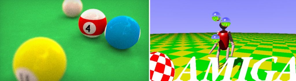
Screen from It's About Time rendered with Brigade 1.

Will wavefront path tracing be faster than its alternative (the megakernel, as Lane and colleagues call it), depends on the time spent in the cores (large scenes and costly shaders reduce the relative excess of costs by the wavefront algorithm), on the maximum path length , mega-core employment and differences in the load on the registers in four stages. In an early version of the original Brigade Path Tracer, we found that even a simple scene with a mix of reflective and Lambert surfaces running on the GTX480 benefited from using wavefront.

Streaming Path Tracing in Lighthouse 2

The Lighthouse 2 platform has two wavefront path tracing tracers. The first one uses Optix Prime for the implementation of stages 2 and 4 (stages of the intersection of rays and the scene); the second uses Optix directly to implement that functionality.

Optix Prime is a simplified version of Optix that only deals with the intersection of a set of rays with a scene consisting of triangles. Unlike the full Optix library, it does not support custom intersection code, and only intersects triangles. However, this is exactly what is required for the wavefront path tracer.

Optix Prime based wavefront path tracer is implemented in rendercore.cpp project. The initialization of Optix Prime starts in the Init function and uses rtpContextCreate . The scene is created using rtpModelCreate . Various ray buffers are created in the SetTarget function using rtpBufferDescCreate . Note that for these buffers we provide the usual device pointers: this means that they can be used both in Optix and in regular CUDA cores.

Rendering begins in the Render method. To fill the primary ray buffer, a CUDA core called generateEyeRays . After filling the buffer, Optix Prime is called using rtpQueryExecute . With it, intersection results are written to extensionHitBuffer . Note that all buffers remain in the GPU: with the exception of kernel calls, there is no traffic between the CPU and GPU. The Shadow phase is implemented in the regular CUDA shade core. Its implementation is in pathtracer.cu .

Some implementation details for optixprime_b are worth mentioning. First, shadow rays are traced outside the wavefront cycle. This is correct: a shadow ray affects a pixel only if it is not blocked, but in all other cases its result is not needed anywhere else. That is, the shadow beam is disposable , it can be traced at any time and in any order. In our case, we use this by grouping the rays of the shadow so that the finally traced batch is as large as possible. This has one unpleasant consequence: with N iterations of the wavefront algorithm and X primary rays, the upper limit of the number of shadow rays is equal to XN .

Another detail is the processing of various counters. The stages “Renew” and “Shadow” should know how many paths are active. Counters for this are updated in the GPU (atomically), which means that they are used in the GPU, even without returning to the CPU. Unfortunately, in one of the cases this is impossible: the Optix Prime library needs to know the number of rays traced. To do this, we need to return the information of the counters once an iteration.

Conclusion

This article explains what wavefront path tracing is and why it is necessary to effectively perform path tracing on the GPU. Its practical implementation is presented in the Lighthouse 2 platform, which is open source and available on Github .