Physics and Economics. Gnoseological difference and its manifestation in IT

I came to the world of IT from theoretical physics. He was mainly engaged in economic tasks. Engaged - this: analysis, TK, statement, design, programming. Naturally, all the time I compared the physical and economic approaches to understanding the laws of nature and economics, respectively. A certain point of view has ripened on this subject. About her and will be discussed.

1. About cognition in general

There are two approaches to cognition:

Aristotle's approach . This is a holistic approach and treats the object as a black box. The phenomenon, the object is studied in all reality as a whole. And reality says, for example, that heavy bodies fall to the ground faster than light ones; that left to itself a moving body gradually stops. Aristotle's approach deals with the phenomenon as an integral reality, and therefore can be called phenomenological.

Galileo's approach . This is an analytical, systems approach. This is the divide and conquer approach. The phenomenon, the object are decomposed into its constituent parts and each of them is studied separately, abstracting from the rest (analysis). Then, the resulting pictures can be combined into one, taking into account the interaction of the components (synthesis). For example, the fall of bodies is considered as the fall of bodies in the void. And there they turn out to fall with the same acceleration. But in reality, friction against air prevents them from falling equally. Having studied this force separately, we can explain the result of Aristotle. Similarly, if we disengage from the forces of friction, then the moving body will move without stopping. And if we take into account the friction force, we get the result of Aristotle. Galileo's approach immediately leads to the need to study forces. This, in the end, translates into a coherent system of classical physics.

Once again, for clarity.

Aristotle's approach . There is a phenomenon under study, “The fall of a body in the air to the ground” - the F. phenomenon. We take different bodies and find that heavier bodies fall to the ground faster than light ones.

Galileo's approach . When studying the phenomenon of F, one must take into account not only weight. We study the fall in the air. And let's change not only weight, but also air. Let's try to reduce its density, so that, in the end, there is no air. Then we find that all bodies fall in the void with the same acceleration. We find the parameters of the effect on the phenomenon and try to create conditions under which only one parameter is significant. This is not in nature. Therefore, a physicist needs a laboratory where he could vary the parameters. Having studied the influence of one parameter, we can proceed to study the influence of another parameter. We are trying to reduce the complexity of the whole approach to the composition of simpler approaches. Varying the shape of the falling body, we can study the dependence of the friction force on air depending on the shape of the body. By varying the rate of fall, we can detect the dependence of the friction force on speed. By varying the height of the fall, we can detect the dependence of acceleration on height. By varying the geographical location on earth, we find the dependence of the acceleration of fall on geography.

Roughly speaking, in the approach of Aristotle they study reality, and in the approach of Galileo they study abstractions, and from them, through synthesis, they go to reality.

2. The model of physical knowledge

Physics is an ideal theory for many sciences, including economics. In physical experiments, discrete series of values ​​are obtained. But they are considered an approximation to continuous functions, which in reality are physical indicators. And physicists are trying to guess these functions. So Galileo guessed the parabola for the trajectory of a stone thrown at an angle to the horizon; Kepler guessed the trajectories of the planets - ellipses, etc. Having guessed the trajectory, we get a predictive apparatus - the ability to calculate the value for unexplored coordinates of the trajectory. To test, they put an experiment - create the conditions for experimental obtaining the value of interest. Then, having verified the predicted value and the experimental one, we get a confirmation or refutation of the theory. Here sometimes the error of the experimental error plays an important role. Physical knowledge comes down to the identification of determinism - the law of obtaining a state from an initial state:

$$

$$S (t) = D (Q, S (0))$$

S(0) -   D –  – ,  S(t)  S(0) Q –       . ,  ,      . 

So, for a thrown stone from a point (0,0) with a speed $$$v_0$at an angle $$$α$to the horizon we have

$$$$ display $$ x (t) = v_0 t cos⁡ (α), y (t) = v_0 t sin⁡ (α) - (gt ^ 2) / 2 $$ display $$

The initial state S (0) is set by three parameters: departure point (0,0), initial speed $$$v_0$angle $$$α$.
The impact of the environment Q is given by the acceleration of gravity g. When expanding the scope of the problem (high initial velocity), g is no longer constant.
The determinism D is given by the above formula.

For a more realistic task, you need to take into account friction against the air. This complicates the math of the problem, but the principle remains the same. Instead of stone, you can consider a plane. Then the thrust force of the aircraft comes into play, and its regulation by the pilot. A non-physical factor also appears - the will of the pilot. We cannot take it into account. But we know that it is not unlimited: traction cannot be infinite, acceleration cannot be infinite. This introduces an element of certainty into the movement. They use it, for example, to build the trajectory of an air defense missile.

Let's go back to the flying stone. It is characterized by an infinite number of physical parameters. For example, only its shape can be arbitrarily complex. But we are sure that in some useful area we can consider the stone as a material point. This is the main abstraction of classical mechanics. All systems are represented as sets of interacting material points. This makes the main cognitive reduction - the reduction of the behavior of a complex system to the behavior of its elementary components.

In connection with the mentioned cognitive reduction, two epistemological approaches can be distinguished - reductionism and holism.

3. Reductionism and holism

Reductionism is the principle of reducing the characteristics of a system from the characteristics of subsystems and the characteristics of the interaction of subsystems. Successfully works in physics.
Consider, for example, gas. Without decomposing it into subsystems, we can operate with experimental, phenomenological concepts: pressure P, temperature T, volume V. Empirically, we find the relation connecting these parameters - the equation of state of the gas:

$$

$$PV = constT$$

This is the so-called phenomenological level - work with phenomena (phenomena) without going into their structure. This is Aristotle's approach.

Now apply the approach of Galileo. We decompose the “gas" system: imagine it as a collection of colliding molecules. Then we define P and T through the mechanical parameters of the molecule. This is done in molecular physics. Thus, we reduce the gas system to subsystems of molecules. This will clarify the equation of state or deduce it for new systems.

Accordingly, in business we have an analogy: macroeconomics are decomposed into enterprises and households. But here the reduction is not yet perfect. Alas, there is no economic Newton. The problem is the complexity and availability of a subjective factor that is not in physics (though there is a debate about the role of the subject in quantum mechanics).

And now about holism.

Holism is the principle that there can be non-reducible properties in a system. So in biology, the doctrine of vitalism is based on the concept of entelechy, the life force inherent in the body as a whole and irreducible.

Physics so far dispenses with the concept of holism.

4. Formula and algorithmic models

A formula model is a model defined by a formula. The concept of “formula” will be considered known.

Examples in physics: Newton equations, Lagrange equations, Maxwell equations, Navier-Stokes equations, Heisenberg-Schrödinger equations, Einstein equations.

Examples from the economy: Black-Scholes formula for the option price, money supply formula, linear programming model for optimizing the financial portfolio, interest calculation formulas, risk calculation formulas.

With a formulaic model, a person can work without a computer. Such is almost all pure mathematics. But here, algorithmic plays an increasingly important role. So the solution to the problem of four colors was not reduced to any formula, but required a brute-force solution for many special cases. This bust was done by computers.

Algorithmic model - a model defined by an algorithm, possibly not reducible to a formula. Of course, it is possible to classify the algorithm as formulas, but these are not the same classical formulas. The algorithmic model is initially realistic only using a computer
A formal model can always be reduced to an algorithmic one.

An example of the first algorithmic model is the Fermi-Pasta-Ulam problem. Here is a quote from Ulam’s book, The Adventures of Mathematics.

And here is an article on Habré, telling about the current state of the Fermi-Pasta-Ulam problem:
Mathematicians solved the Fermi-Pasta-Ulam problem

5. Coordination

By system coordination, I understand the definition of basic parameters, which in principle determine the evolution of the system. For example, in the mechanics of a material point, the coordination is defined by:

• External force F
  
  • Mass m material point
  • Spatial coordinates (x, y, z) = r of the material point
  • Time t

The evolution of the system is given by Newton's equation

$$

$$(d ^ 2 r (t)) / (dt ^ 2) = (F (t)) / m$$

What is the coordination of the economic entity? I once worked on a business intelligence system. Its main term is indicator. The basis of the system is a scorecard. Hundreds of indicators. But I searched in vain on the Internet for a description of the basis of indicators - a set of indicators that cannot be reduced to others and which, in principle, completely determine the evolution of an economic entity. That is, as I understand it, no coordination has been made in the economy. And, therefore, talking about some basic dynamic law is not yet possible. It is only possible, based on the connection of indicators, to conduct a scenario analysis - to answer the question “What will happen to the derived indicators if the underlying indicators will change according to the given scenario?”

6. Abstract example. Time Series Forecasting Like Physics

You can ask the forecasting problem based on the actual time series: having a number of real values, you need to get the predicted value of the indicator - the value in the future. This suggests a kind of hidden determinism of the time series. There were many scientific and pseudo-scientific speculations on this subject. I myself dealt with doctors of sciences who claimed that their methodology would allow them to obtain an exchange rate forecast and showed the corresponding dissertations with all sorts of confidence intervals and other attributes of distribution laws. But, when confronted with reality, the techniques were blown away.

Sometimes to get a forecast do this:

1. Take the real time series {V (ti)}. Schedule - step broken line.
2. Take a continuous function W (t) such that W (ti) = V (ti). The graph is a continuous curve.
3. A polynomial P (t) is selected that approximates W (t) with a sufficient degree of accuracy. A polynomial can be considered for all t.
4. Then we have a forecast for future time T: V (T) = P (T)
   All this gives the impression of science, but only at first glance. Yes, the existence of an approximating polynomial for W (t) is guaranteed by the Weierstrass theorem from matanalysis. We can polynomize W (t) arbitrarily precisely. But it cannot be used for predictions.

The approximative value for the real series is 100%, and the predictive value is zero. Polynomials can be invented arbitrarily, but they will all give different forecasts.

When day T arrives and we find out the real V (T), then for the series {{V (ti)}, V (T)} we can construct a new polynomial Q (t) which approximates this series arbitrarily exactly, but the time T is no longer in the future and Q (T) is no longer a forecast, but a reality. The polynomials P (t) and Q (t) absolutely do not have to coincide, and for the new forecast time T '> T they will show different results. That is, there is no forecast. There seems to be science, but no forecast. This is like the medieval theory of angels. She can explain everything, but she cannot predict anything.

The difference between physical interpolation and extrapolation from economic:

• The accuracy of empirical data : approximate in physics, accurate in economics
• Domain functions : continuous in physics, discontinuous, stepwise in economics
• Empirical data : in physics, discrete, in economics continuous with discrete discontinuities
• Basic laws : in physics there. F = ma, for example; in the economy yet

7. Economics and physics

In economics, real trajectories — essentially discontinuous — are piecewise constant functions. For example, the “Currency rate” indicator can make a jump at any time. Continuous economic functions - approximations for the sake of matanalysis (if you have a hammer in your hands, then you want to consider any object as a nail ...). Each accounting transaction causes jumps in the values ​​of indicators of derivatives from accounts. And they are the majority of indicators. Further, each change in the number of workers is discrete, etc. The continuity of economic trajectories contrasts with the continuity of most physical trajectories. Therefore, the apparatus of matanalysis is not directly applicable to economic trajectories.

Picture for physical cognition. The trajectory of a stone thrown at an angle to the horizon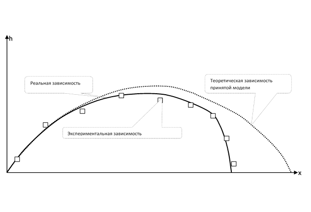

Picture for economic knowledge. The exchange rate at the central bank.

This is a real experimental exact function. It is discontinuous at points in time when the exchange rate changes.

In physics:

• Experimental physical values ​​are almost always approximate
• Experimental physical values ​​form a discrete series.
• The experimental discrete series is considered as a polygon for continuous approximation because reality is continuous. The notion of continuity may turn out to be a lie on small spatial and temporal scales. Then physics will change its face.
• Well defined baseline indicators
• Theoretical and real trajectories are almost always continuous and almost always differentiable (the trajectory of a material point is always twice differentiable in time)
• Due to the continuity of real dynamics and the real trajectory, its good continuous approximation has predictive power: in a sufficiently small neighborhood, the function will not go far from its last real value.

In economics:

• Experimental economic values ​​can be considered accurate. Only in macroeconomics is there a problem of accuracy due to the huge number of business entities.
• Experimental economic values ​​consist of intervals of constancy, interrupted at certain points in time when the value changes abruptly
• Experimental data cannot be considered as a testing ground for continuous approximation because reality is discontinuous.
• Not fully defined baseline indicators. It is not clear why to dance.
• Due to the discontinuity of the real trajectory, any arbitrarily good continuous approximation of it does not guarantee predictions in any arbitrarily small neighborhood.
• Real trajectories are almost always discontinuous. This means that economic determination requires an approach different from classical mechanics.
• In the economy, there is initially a factor of free will of an economic entity. Its range is regulated by the state. The extreme limits of this freedom:
  - Complete freedom in a non-state-regulated market
  - Partial freedom in a partially regulated market
  - Complete lack of freedom in a totally centralized state where there is no free market

Economic knowledge has not reached a level similar to classical mechanics:

2. Q( ), , ,
3. ,
4. ; .

. – . – . ? , . . . . , – .

, . , , - .

8. IT

8.1.

. . . . , . . . . . . . , , . . … , . It's enough. , . . . , . . . . . . . . . . . – " . - "!? , . -1840( , ). . . , . , . , . , . On that and parted. , , . (). . , , , : ", . ". ! . , , - .

8.2. -

. — . , , .. . . , . . – . , . , . – . . …

. . , . , , , . , . . . . . , - . . . . , : , . . . , , . . ? . . , .

. - , .

, , . , . . , .

. . . , . , . , : , . , . . .

, – Jump Processing. , . But this is a completely different story.

, . “ ”. , – . , , . – , . . , – .

8.3.

( ). . “”. . , . , . . – . . , . . . . , . . – . . , . … . ? , . , - . . . , . , , . . .

. , . , . , – . , . , – ( – ?).

8.4.

_{“ ”}

. () . . . , , . . , . . , , . . . – . , , . , . . , . Handsomely. . – . , . – . . , (, ). , . . , . . , , , . . . – . . . . . . . . . : , , , , , , , , … . 100 . ( , , ) . , ( , (SQL-) ). , . Those. . . . , . . , : ”, . . . ”.

. , . , . : . , , .

. . . , , . . . . -.

() . , , ( ), . , . , – . , , , , , . . . , , . , “” “”. , “” “”. ? , .

: . . . , . . . . — . . : . : , …

. . , . . Which is to be expected.

Summary

, . . - . . — . ? .

: IT. .