We write a simple neural network using mathematics and numpy

Why another article about how to write neural networks from scratch? Alas, I could not find an article where theory and code would be described from scratch to a fully working model. Immediately I warn you that there will be a lot of mathematics. I assume that the reader is familiar with the basics of linear algebra, partial derivatives and at least partially, with probability theory, as well as Python and Numpy. We will deal with a fully connected neural network and MNIST.

Maths. Part 1 (simple)

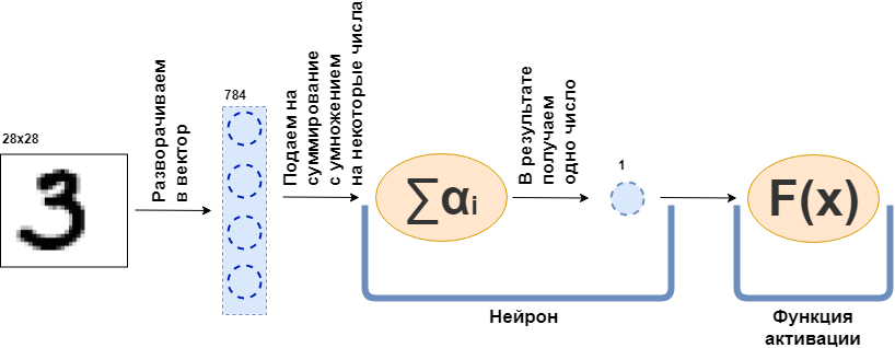
What is a fully connected layer (FC layer)? Usually they say something in the spirit of "A fully connected layer is a layer, each neuron of which is connected to all the neurons of the previous layer." That's just not clear what neurons are, how they are connected, especially in the code. Now I will try to make out this example. So let there be a layer of 100 neurons. I know that I have not yet explained what it is, but let's just imagine that there are 100 neurons and they have an input, where the data are being fed, and an output, from where they give out data. And at the input they are given a black and white picture of 28x28 pixels - only 784 values, if you stretch it into a vector. The picture can be called the input layer. Then each of the 100 neurons connects with each “neuron” or, if you like, the value of the previous layer (that is, the picture), each of the 100 neurons needs to accept 784 values ​​of the original picture. For example, for each of the 100 neurons it will be enough to multiply 784 values ​​of the image by some 784 numbers and add them together, as a result one number comes out. That is, this is the neuron:

$$$$ display $$ \ text {Neuron output} = \ text {some number} _ {1} \ cdot \ text {picture value} _1 ~ + \\ + ~ ... ~ + ~ \ text {some then number} _ {784} \ cdot \ text {picture value} _ {784} $$ display $$

Then it turns out that each neuron has 784 numbers, and all of these numbers: (number of neurons on this layer) x (number of neurons on the previous layer) =$$ $ inline $ 100 \ times784 $ inline $ = 78 400 digits. These numbers are usually called layer weights. Each neuron will produce its own number and as a result we will get a 100-dimensional vector, and in fact we can write that this 100-dimensional vector is obtained by multiplying a 784-dimensional vector (our original image) by a matrix of weights$$ $ inline $ 100 \ times784 $ inline $ :

$$$$ display $$ \ boldsymbol {x} ^ {100} = W_ {100 \ times784} \ cdot \ boldsymbol {x} ^ {784} $$ display $$

Next, the resulting 100 numbers are passed on to the activation function — some non-linear function — that affects each number of series. For example, sigmoid, hyperbolic tangent, ReLU and others. The activation function is necessarily non-linear, otherwise the neural network will learn only simple transformations.


')
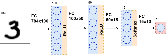
Then the resulting data is again fed to the fully connected layer, but with a different number of neurons, and again to the activation function. This happens several times. The last layer of the network is the layer that gives the answer. In this case, the answer is information about the number in the picture.



During the training of the network, it is necessary that we know what figure is shown in the picture. That is, to be marked up. Then you can use another element - the error function. She looks at the neural network's response and compares with the real answer. Thanks to this neural network and learns.

General formulation of the problem

The whole dataset is a large tensor (we will call a multidimensional data array as a tensor)$$ $ inline $ \ boldsymbol {X} = \ left [\ boldsymbol {x} _1, \ boldsymbol {x} _2, \ ldots, \ boldsymbol {x} _n \ right] $ inline $ where$$ $ inline $ \ boldsymbol {x} _i $ inline $ - i-th object, for example, a picture, which is also a tensor. For each object there is$$ $ inline $ y_i $ inline $ - the correct answer on the i-th object. In this case, the neural network can be represented as a certain function that accepts an object as input and outputs some answer on it:

$$$$ display $$ F (\ boldsymbol {x} _i) = \ hat {y} _i $$ display $$

Now let's take a closer look at the function$$ $ inline $ F (\ boldsymbol {x} _i) $ inline $ . Since the neural network consists of layers, each individual layer is a function. Which means

$$$$ display $$ F (\ boldsymbol {x} _i) = f_k (f_ {k-1} (\ ldots (f_1 (\ boldsymbol {x} _i)))) = \ hat {y} _i $$ display $ $

That is, in the very first function - the first layer - a picture is fed in the form of a certain tensor. Function$$ $ inline $ f_1 $ inline $ gives some answer - also a tensor, but of a different dimension. This tensor will be called an internal representation. Now this internal representation is input to the function.$$ $ inline $ f_2 $ inline $ , which gives its internal presentation. And so on, while the function$$ $ inline $ f_k $ inline $ - the last layer - will not give an answer$$ $ inline $ \ hat {y} _i $ inline $ .

Now, the task is to train the network - to make the network response coincide with the correct answer. First you need to measure how wrong the neural network is. This will be measured by the error function.$$ $ inline $ L (\ hat {y} _i, y_i) $ inline $ . And we impose restrictions:

one.$$ $ inline $ \ hat {y} _i \ xrightarrow {} y_i \ Rightarrow L (\ hat {y} _i, y_i) \ xrightarrow {} 0 $ inline $
2$$ $ inline $ \ exists ~ dL (\ hat {y} _i, y_i) $ inline $
3$$ $ inline $ L (\ hat {y} _i, y_i) \ geq 0 $ inline $

Restriction 2 impose on all functions of layers$$ $ inline $ f_j $ inline $ - let them all be differentiable.

Moreover, in fact (about this, I omitted) some of these functions depend on the parameters - the weights of the neural network -$$ $ inline $ f_j (\ boldsymbol {x} _i | \ boldsymbol {\ omega} _j) $ inline $ . And the whole idea is to pick such weights to$$ $ inline $ \ hat {y} _i $ inline $ coincided with$$ $ inline $ y_i $ inline $ on all objects dataset. I note that the weight is not in all functions.

So where are we staying? All functions of the neural network are differentiable, the error function is also differentiable. Recall one of the properties of the gradient - to show the direction of growth of the function. We take advantage of this, restrictions 1 and 3, the fact that

$$$$ display $$ L (F (\ boldsymbol {x} _i)) = L (f_k (f_ {k-1} (\ ldots (f_1 (\ boldsymbol {x} _i))))) = L (\ hat {y} _i) $$ display $$

and the fact that I can count partial derivatives and derivatives of a complex function. Now there is everything you need in order to calculate

$$$$ display $$ \ frac {\ partial L (F (\ boldsymbol {x} _i))} {\ partial \ boldsymbol {\ omega_j}} $$ display $$

for any i and j. This partial derivative indicates the direction in which you want to change$$ $ inline $ \ boldsymbol {\ omega_j} $ inline $ to increase$$ $ inline $ L $ inline $ . To reduce the need to take a step towards$$ $ inline $ - \ frac {\ partial L (F (\ boldsymbol {x} _i))} {\ partial \ boldsymbol {\ omega_j}} $ inline $ nothing complicated.

So the network learning process is built like this: several times in a cycle we go through the whole dataset (this is called an era), for each object we consider$$ $ inline $ L (\ hat {y} _i, y_i) $ inline $ (this is called forward pass) and consider the partial derivative$$ $ inline $ \ partial L $ inline $ for all scales$$ $ inline $ \ boldsymbol {\ omega_j} $ inline $ then weights are updated (this is called backward pass).

I note that I have not yet introduced any specific functions and layers. If at this stage it is not entirely clear what to do with all this, I suggest that you continue reading - there will be more mathematics, but now it will come with examples.

Maths. Part 2 (complicated)

Error function

I will start at the end and output the error function for the classification problem. For the regression problem, the output of the error function is well described in the book Deep Learning. Immersion in the world of neural networks.

For simplicity, there is a neural network (NN) that separates photos of cats from photos of dogs, and there is a set of photos of cats and dogs for which there is a correct answer.$$ $ inline $ y_ {true} $ inline $ .

$$$$ display $$ NN (picture | \ Omega) = y_ {pred} $$ display $$

All that I will do next is very similar to the maximum likelihood method. Therefore, the main task is to find the likelihood function. If we omit the details, then such a function that matches the prediction of the neural network and the correct answer, and if they match, gives a great value, if not, on the contrary. The probability of a correct answer comes to mind with the given parameters:

$$$$ display $$ p (y_ {pred} = y_ {true} | \ Omega) $$ display $$

And now we will make some trick that does not seem to follow from anywhere. Let the neural network produce a response in the form of a two-dimensional vector, the sum of which is 1. The first element of this vector can be called the measure of confidence that the photo is a cat, and the second element the measure of confidence that the photo is a dog. Yes, it's almost likelihood!

$$$$ display $$ NN (picture | \ Omega) = \ left [\ begin {matrix} p_0 \\ p_1 \\\ end {matrix} \ right] $$ display $$

Now the likelihood function can be rewritten in the form:

$$$$ display $$ p (y_ {pred} = y_ {true} | \ Omega) = p_ \ Omega (y_ {pred}) ^ t_ {0} * (1 - p_ \ Omega (y_ {pred})) ^ t_ {1} = \\ p_0 ^ {t_0} * p_1 ^ {t_1} $$ display $$

Where$$ $ inline $ t_0, t_1 $ inline $ tags of the right class, for example, if$$ $ inline $ y_ {true} = cat $ inline $ then$$ $ inline $ t_0 == 1, t_1 == 0 $ inline $ , if a$$ $ inline $ y_ {true} = dog $ inline $ then$$ $ inline $ t_0 == 0, t_1 == 1 $ inline $ . Thus, the probability of a class that should have been predicted by the neural network (but not necessarily predicted by it) is always considered. Now it can be generalized to any number of classes (for example, m classes):

$$$$ display $$ p (y_ {pred} = y_ {true} | \ Omega) = \ prod_0 ^ m p_i ^ {t_i} $$ display $$

However, in any dataset there are many objects (for example, N objects). It would be desirable, that on each or the majority of objects the neural network would give the correct answer. And for this you need to multiply the results of the formula above for each object from the dataset.

$$$$ display $$ MaximumLikelyhood = \ prod_ {j = 0} ^ N \ prod_ {i = 0} ^ m p_ {i, j} ^ {t_ {i, j}} $$ display $$

To get good results, this function must be maximized. But, first, to minimize steeper, because we have a stochastic gradient descent and all the buns for it - we simply assign a minus, and, secondly, it is difficult to work with a huge work - logarithmically.

$$$$ display $$ CrossEntropyLoss = - \ sum \ limits_ {j = 0} ^ {N} \ sum \ limits_ {i = 0} ^ {m} t_ {i, j} \ cdot \ log (p_ {i, j }) $$ display $$

Wonderful! The result is cross-entropy or, in the binary case, logloss. This function is easy to read and even easier to differentiate:

$$$$ display $$ \ frac {\ partial CrossEntropyLoss} {\ partial p_j} = - \ frac {\ boldsymbol {t_j}} {\ boldsymbol {p_ {j}}} $$ display $$

It is necessary to differentiate for the back-propagation error algorithm. I note that the error function does not change the dimension of the vector. If, as in the case of MNIST, the output is a 10-dimensional vector of answers, then when calculating the derivative we get a 10-dimensional vector of derivatives. Another interesting thing is that only one element of the derivative will not be zero, where$$ $ inline $ t_ {i, j} \ neq 0 $ inline $ , that is, with the right answer. And the less likely the correct answer is predicted neural network on this object, the more it will be the error function.

Activation functions

At the output of each fully connected layer of the neural network, a nonlinear activation function must be present. Without it, it is impossible to train a content neural network. If you run ahead, the fully connected layer of the neural network is simply a multiplication of the input data by a matrix of weights. In linear algebra, this is called a linear mapping — some linear function. The combination of linear functions is also a linear function. But this means that such a function can approximate only linear functions. Alas, this is not why neural networks are needed.

Softmax

Usually this function is used on the last layer of the network, since it turns the vector from the last layer into a vector of “probabilities”: each element of the vector lies from 0 to 1 and their sum is 1. It does not change the dimension of the vector.

$$$$ display $$ Softmax_i = \ frac {e ^ {x_i}} {\ sum \ limits_ {j} e ^ {x_j}} $$ display $$

We now turn to the search for a derivative. Because$$ $ inline $ \ boldsymbol {x} $ inline $ Is a vector, and all its elements are always present in the denominator, then taking a derivative we get Jacobians:

$$$$ display $$ J_ {Softmax} = \ begin {cases} x_i - x_i \ cdot x_j, i = j \\ - x_i \ cdot x_j, i \ neq j \ end {cases} $$ display $$

Now about backpropagation. From the previous layer (usually the error function) comes the vector of derivatives$$ $ inline $ \ boldsymbol {dz} $ inline $ . If$$ $ inline $ \ boldsymbol {dz} $ inline $ came from the error function on MNIST,$$ $ inline $ \ boldsymbol {dz} $ inline $ - 10-dimensional vector. Then the Jacobian has a dimension of 10x10. To obtain$$ $ inline $ \ boldsymbol {dz_ {new}} $ inline $ which will go further to the previous layer (do not forget that we go from the end to the beginning of the network when the error propagates back), we need to multiply$$ $ inline $ \ boldsymbol {dz} $ inline $ on$$ $ inline $ J_ {Softmax} $ inline $ (row per column):

$$$$ display $$ dz_ {new} = \ boldsymbol {dz} \ times J_ {Softmax} $$ display $$

The output is a 10-dimensional vector of derivatives$$ $ inline $ \ boldsymbol {dz_ {new}} $ inline $ .

Relu

$$$$ display $$ ReLU (x) = \ begin {cases} x, x> 0 \\ 0, x <0 \ end {cases} $$ display $$

ReLU began to be massively used after 2011, when the article “Deep Sparse Rectifier Neural Networks” was published. However, such a function was known before. Such a concept as “activation force” is applicable to ReLU (for more information about this, read the book Deep Learning. Immersion in the World of Neural Networks). But the main feature that makes ReLU more attractive than other activation functions is a simple calculation of the derivative:

$$$$ display $$ d (ReLU (x)) = \ begin {cases} 1, x> 0 \\ 0, x <0 \ end {cases} $$ display $$

Thus, ReLU is computationally more efficient than other activation functions (sigmoid, hyperbolic tangent, etc.).

Full connected layer

Now is the time to discuss the fully connected layer. The most important of all the others, because it is in this layer that all the weights are found that need to be adjusted in order for the neural network to work well. A fully connected layer is simply a matrix of weights:

$$$$ display $$ W = | w_ {i, j} | $$ display $$

A new internal representation is obtained when the weights matrix is ​​multiplied by the input column:

$$$$ display $$ \ boldsymbol {x} _ {new} = W \ cdot \ boldsymbol {x} $$ display $$

Where$$ $ inline $ \ boldsymbol {x} $ inline $ has a size$$ $ inline $ input \ _shape $ inline $ , but$$ $ inline $ x_ {new} $ inline $ -$$ $ inline $ output \ _shape $ inline $ . For example,$$ $ inline $ \ boldsymbol {x} $ inline $ - 784-dimensional vector, and$$ $ inline $ \ boldsymbol {x} _ {new} $ inline $ - 100-dimensional vector, then the matrix W has a size of 100x784. It turns out that on this layer is 100x784 = 78,400 weights.

When back propagating an error, you need to take the derivative with respect to each weight of this matrix. Simplify the problem and take only the derivative with respect to$$ $ inline $ w_ {1,1} $ inline $ . When multiplying the matrix and vector, the first element of the new vector$$ $ inline $ \ boldsymbol {x} _ {new} $ inline $ equals$$ $ inline $ x_ {new ~ 1} = w_ {1,1} \ cdot x_1 + ... + w_ {1,784} \ cdot x_ {784} $ inline $ and derivative$$ $ inline $ x_ {new ~ 1} $ inline $ by$$ $ inline $ w_ {1,1} $ inline $ will be just$$ $ inline $ x_1 $ inline $ , you just need to take the derivative of the amount above. Similarly, for all other scales. But this is not yet an algorithm for back-propagating an error, as long as it is just a matrix of derivatives. It is necessary to remember that from the next layer this (the error goes from the end to the beginning) comes a 100-dimensional gradient vector$$ $ inline $ d \ boldsymbol {z} $ inline $ . The first element of this vector$$ $ inline $ dz_1 $ inline $ will be multiplied by all elements of the derivative matrix that “participated” in creating$$ $ inline $ x_ {new ~ 1} $ inline $ that is to$$ $ inline $ x_1, x_2, ..., x_ {784} $ inline $ . Similarly, the other elements. If we translate it into the language of linear algebra, then it is written as:

$$$$ display $$ \ frac {\ partial L} {\ partial W} = (d \ boldsymbol {z}, ~ dW) = \ left (\ begin {matrix} dz_ {1} \ cdot \ boldsymbol {x} \ \ ... \\ dz_ {100} \ cdot \ boldsymbol {x} \ end {matrix} \ right) _ {100} $$ display $$

The output is a matrix of 100x784.


Now you need to understand what to transfer to the previous layer. For this and for a greater understanding of what actually happened now, I want to write down what happened when taking the derivatives on this layer in a slightly different language, moving away from the specifics of “what is multiplied by” to the functions (again).

When I wanted to adjust the weights, I wanted to take the derivative of the error function on these weights:$$ $ inline $ \ frac {\ partial L} {\ partial W} $ inline $ . Above it was shown how to derive derivatives with respect to error functions and activation functions. Therefore, we can consider the following case (in$$ $ inline $ d \ boldsymbol {z} $ inline $ all derivatives of the error function and activation functions are already sitting):

$$$$ display $$ \ frac {\ partial L} {\ partial W} = d \ boldsymbol {z} \ cdot \ frac {\ partial \ boldsymbol {x} _ {new} (W)} {\ partial W} $ $ display $$

This can be done because you can consider$$ $ inline $ \ boldsymbol {x} _ {new} $ inline $ , as a function of W:$$ $ inline $ \ boldsymbol {x} _ {new} = W \ cdot \ boldsymbol {x} $ inline $ .
You can substitute this in the formula above:

$$$$ display $$ \ frac {\ partial L} {\ partial W} = d \ boldsymbol {z} \ cdot \ frac {\ partial W \ cdot \ boldsymbol {x}} {\ partial W} = d \ boldsymbol { z} \ cdot E \ cdot \ boldsymbol {x} $$ display $$

Where E is the matrix consisting of units (NOT the identity matrix).

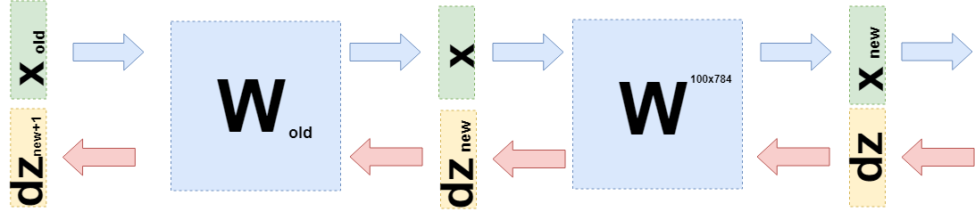
Now when you need to take a derivative of the previous layer (even for simplicity of calculations, this will also be a fully connected layer, but in general it does not change anything), then you need to consider$$ $ inline $ \ boldsymbol {x} $ inline $ as a function of the previous layer$$ $ inline $ \ boldsymbol {x} (W_ {old}) $ inline $ :

$$$$ display $$ \ begin {gathered} \ frac {\ partial L} {\ partial W_ {old}} = d \ boldsymbol {z} \ cdot \ frac {\ partial \ boldsymbol {x} _ {new} (W )} {\ partial W_ {old}} = d \ boldsymbol {z} \ cdot \ frac {\ partial W \ cdot \ boldsymbol {x} (W_ {old})} {\ partial W_ {old}} = \\ = d \ boldsymbol {z} \ cdot \ frac {\ partial W \ cdot W_ {old} \ cdot \ boldsymbol {x} _ {old}} {\ partial W_ {old}} = d \ boldsymbol {z} \ cdot W \ cdot E \ cdot \ boldsymbol {x} _ {old} = \\ = d \ boldsymbol {z} _ {new} \ cdot E \ cdot \ boldsymbol {x} _ {old} \ end {gathered} $$ display $$

Exactly$$ $ inline $ d \ boldsymbol {z} _ {new} = d \ boldsymbol {z} \ cdot W $ inline $ and need to send to the previous layer.

Code

First of all, this article is aimed at explaining the mathematics of neural networks. I will give the code quite a bit of time.

This is an example of the implementation of the error function:

class CrossEntropy: def forward(self, y_true, y_hat): self.y_hat = y_hat self.y_true = y_true self.loss = -np.sum(self.y_true * np.log(y_hat)) return self.loss def backward(self): dz = -self.y_true / self.y_hat return dz 

The class has methods for forward and backward pass. At the time of a straight pass, an instance of the class saves the data inside the layer, and at the time of the back pass it uses them to calculate the gradient. The rest of the layers are constructed in the same way. This makes it possible to write a fully connected neural in this style:

 class MnistNet: def __init__(self): self.d1_layer = Dense(784, 100) self.a1_layer = ReLu() self.drop1_layer = Dropout(0.5) self.d2_layer = Dense(100, 50) self.a2_layer = ReLu() self.drop2_layer = Dropout(0.25) self.d3_layer = Dense(50, 10) self.a3_layer = Softmax() def forward(self, x, train=True): ... def backward(self, dz, learning_rate=0.01, mini_batch=True, update=False, len_mini_batch=None): ... 

The full code can be found here .
Also I advise to study this article on Habré .

Conclusion

I hope I was able to explain and show that quite simple mathematics is behind neural networks and that it is absolutely not scary. Nevertheless, for a deeper understanding, it is worth trying to write your own “bicycle”. Corrections and suggestions are happy to read in the comments.