The book "Machine learning for business and marketing"

Data science is becoming an integral part of any marketing activity, and this book is a living portrait of digital transformations in marketing. Data analysis and intelligent algorithms automate time-consuming marketing tasks. The decision-making process becomes not only more perfect, but also faster, which is of great importance in a constantly accelerating competitive environment.

“This book is a living portrait of digital transformations in marketing. It shows how data science becomes an integral part of any marketing activity. It describes in detail how approaches based on data analysis and intelligent algorithms contribute to the deep automation of traditionally labor-intensive marketing tasks. The decision-making process is becoming not only more perfect, but also faster, which is important in our constantly accelerating competitive environment. This book must be read by data processing specialists and marketing specialists, and it’s better if they read it together. ”Andrey Sebrant, director of strategic marketing, Yandex.

Excerpt 5.8.3. Hidden factors models

In the joint filtering algorithms discussed so far, most of the calculations are performed on the basis of individual elements of the rating matrix. Proximity-based methods estimate missing ratings directly from known values ​​in the rating matrix. Model-based methods add an abstraction layer on top of the rating matrix, creating a predictive model that captures certain patterns in the relationship between users and elements, but the training of the model is still highly dependent on the properties of the rating matrix. As a result, these methods of co-filtering usually face the following problems:

The matrix of ratings can contain millions of users, millions of elements and billions of known ratings, which creates serious problems of computational complexity and scalability.
')
The matrix of ratings, as a rule, is very rarefied (in practice, about 99% of ratings may be absent). This affects the computational stability of the recommendation algorithms and leads to unreliable estimates when the user or the element has no really similar neighbors. This problem is often exacerbated by the fact that most of the basic algorithms are focused either on users or on elements, which limits their ability to capture all types of similarities and relationships available in the rating matrix.

The data in the rating matrix is ​​usually highly correlated due to the similarities of users and items. This means that the signals available in the rating matrix are not only sparse, but also redundant, which exacerbates the scalability problem.

The above considerations indicate that the original matrix of ratings may not be the most optimal representation of signals, and other alternative representations that are more suitable for co-filtering purposes should be considered. To explore this idea, let’s go back to the starting point and think a bit about the nature of recommendation services. In essence, a recommendation service can be viewed as an algorithm that predicts ratings based on some measure of similarity between the user and the element:


One way to determine this measure of similarity is to use the approach of hidden factors and map users and elements to points in a certain k-dimensional space so that each user and each element is represented by a k-dimensional vector:


Vectors should be constructed so that the corresponding dimensions p and q are comparable with each other. In other words, each dimension can be considered as a sign or concept, that is, puj is a measure of the proximity of the user u and the concept of j, and qij, respectively, is a measure of the element i and the concept of j. In practice, these dimensions are often interpreted as genres, styles, and other attributes that apply simultaneously to users and elements. The similarity between the user and the element and, accordingly, the rating can be defined as the product of the corresponding vectors:


Since each rating can be decomposed into a product of two vectors belonging to a concept space that is not directly observed in the initial rating matrix, p and q are called hidden factors. The success of this abstract approach, of course, depends entirely on how the hidden factors are defined and constructed. To answer this question, we note that expression 5.92 can be rewritten in a matrix form as follows:


where P is an n × k matrix assembled from vectors p, and Q is an m × k matrix assembled from q vectors, as shown in Fig. 5.13. The main goal of the collaborative filtering system is usually to minimize the error of rating prediction, which allows us to directly define the optimization problem relative to the matrix of hidden factors:



If we assume that the number of hidden dimensions k is fixed and k ≤ n and k ≤ m, the optimization problem 5.94 reduces to the low-rank approximation problem, which we considered in Chapter 2. To demonstrate the approach to the solution, let us assume for a moment that the rating matrix is ​​complete. In this case, the optimization problem has an analytical solution in terms of singular decomposition (Singular Value Decomposition, SVD) of the rating matrix. In particular, using the standard SVD algorithm, the matrix can be decomposed into the product of three matrices:


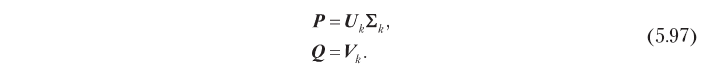
where U is an n × n matrix orthonormal in columns, Σ is a n × m diagonal matrix, and V is an m × m matrix orthonormal in columns. The optimal solution of problem 5.94 can be obtained in terms of these factors, truncated to k of the most significant dimensions:


Consequently, hidden factors that are optimal in terms of prediction accuracy can be obtained by singular decomposition, as shown below:


This model of hidden factors, based on SVD, helps to solve the problems of co-filtering described in the beginning of the section. First, it replaces a large matrix of n × m ratings with matrices of n × k and m × k factors, which are usually much smaller, because in practice the optimal number of hidden dimensions k is often small. For example, there is a case in which the rating matrix with 500,000 users and 17,000 elements was fairly well approximated using 40 measurements [Funk, 2016]. Further, SVD eliminates the correlation in the matrix of ratings: the matrix of hidden factors, defined by the expression 5.97, are orthonormal in columns, that is, the hidden measurements are not correlated. If, which is usually true in practice, SVD also solves the problem of sparseness, because the signal present in the original rating matrix is ​​effectively concentrated (remember that we choose the k dimensions with the highest signal energy) and the matrix of hidden factors are not sparse. Figure 5.14 illustrates this property. The proximity-based user-based algorithm (5.14, a) collapses the sparse rating vectors for a given element and a given user to get a rating score. The model of hidden factors (5.14, b), on the contrary, estimates the rating by convolving two vectors of reduced dimension and with a higher energy density.


The approach just described looks like a well-balanced solution to the problem of hidden factors, but in fact it has a serious disadvantage due to the assumption of the completeness of the rating matrix. If the rating matrix is ​​sparse, which is almost always the case, the standard SVD algorithm cannot be applied directly, since it is not able to handle the missing (undefined) elements. The simplest solution in this case is to fill the missing ratings with some default value, but this can lead to a serious shift in the forecast. Moreover, it is inefficient from a computational point of view, because the computational complexity of such a solution is equal to the SVD complexity for the full n × m matrix, while it is desirable to have a method with complexity proportional to the number of known ratings. These problems can be solved using the alternative decomposition methods described in the following sections.

5.8.3.1. Decomposition without limits

The standard SVD algorithm is an analytical solution to the problem of low-rank approximation. However, this problem can be viewed as an optimization problem, and universal optimization methods can also be applied to it. One of the simplest approaches is to use the gradient descent method to iteratively refine the values ​​of hidden factors. The starting point is to determine the cost function J as a residual forecast error:


Note that this time we do not impose any restrictions, such as orthogonality, on the matrix of hidden factors. Calculating the gradient of the cost function with respect to hidden factors, we get the following result:


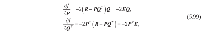
where E is the residual error matrix:


The gradient descent algorithm minimizes the cost function by moving at each step in the negative direction of the gradient. Therefore, it is possible to find hidden factors that minimize the square of the error in forecasting the rating by iteratively changing the matrices P and Q to convergence, in accordance with the following expressions:


where α is the learning rate. The disadvantage of the gradient descent method is the need to calculate the entire matrix of residual errors and simultaneously change all the values ​​of the hidden factors in each iteration. An alternative approach, which may be better suited for large matrices, is stochastic gradient descent [Funk, 2016]. The stochastic gradient descent algorithm uses the fact that the total prediction error J is the sum of errors for individual elements of the rating matrix, so the general gradient J can be approximated by a gradient at one data point and alter the hidden factors elementwise. The full realization of this idea is shown in algorithm 5.1.


The first stage of the algorithm is the initialization of matrices of hidden factors. The choice of these initial values ​​is not very important, but in this case the uniform distribution of the energy of the known ratings among randomly generated hidden factors is chosen. The algorithm then sequentially optimizes the dimensions of the concept. For each measurement, he repeatedly rounds up all ratings in the training set, predicts each rating using the current values ​​of the hidden factors, estimates the error and adjusts the values ​​of the factors in accordance with expressions 5.101. The optimization of the measurement is completed by the condition of convergence, after which the algorithm proceeds to the next measurement.

Algorithm 5.1 helps overcome the limitations of the standard SVD method. It optimizes hidden factors by cycling through individual data points, and thus avoids problems with missing ratings and algebraic operations with giant matrices. The iterative approach also makes stochastic gradient descent more convenient for practical applications than gradient descent, which modifies whole matrices with expressions 5.101.

EXAMPLE 5.6

In essence, the approach based on hidden factors is a whole group of methods for teaching perceptions that can identify patterns that are implicitly present in the rating matrix and represent them explicitly in the form of concepts. Sometimes concepts have a quite meaningful interpretation, especially high-energy ones, although this does not mean that all concepts always have a meaningful meaning. For example, the application of the matrix decomposition algorithm to a movie rating database can create factors approximately corresponding to psychographic measurements, such as melodrama, comedy, a horror film, etc. We illustrate this phenomenon with a small numerical example that uses the rating matrix from Table. 5.3:


First, we subtract the global mean μ = 2.82 from all the elements to center the matrix, and then we perform the algorithm 5.1 with k = 3 hidden measurements and the learning rate α = 0.01 to get the following two matrixes of factors:


Each row in these matrices corresponds to a user or movie, and all 12 row vectors are depicted in Figure. 5.15. Note that the elements in the first column (the first vector of concepts) have the largest values, and the values ​​in the subsequent columns gradually decrease. This is explained by the fact that the first vector concept captures as much signal energy as possible using one dimension, the second vector concept captures only part of the residual energy, etc. Further, note that the first concept can be semantically interpreted as the drama axis - action movie, where the positive direction corresponds to the genre of the action movie, and the negative direction - to the genre of drama. The ratings in this example have a high correlation, so it is clearly seen that the first three users and the first three films have large negative values ​​in the first vector-concept (drama films and users who like such films), while the last three users and the last three films have large positive values ​​in the same column (action films and users who prefer this genre). The second dimension in this particular case corresponds mainly to the bias of the user or element, which can be interpreted as a psychographic attribute (is the criticality of the user's judgment? Film popularity?). The remaining concepts can be regarded as noise.


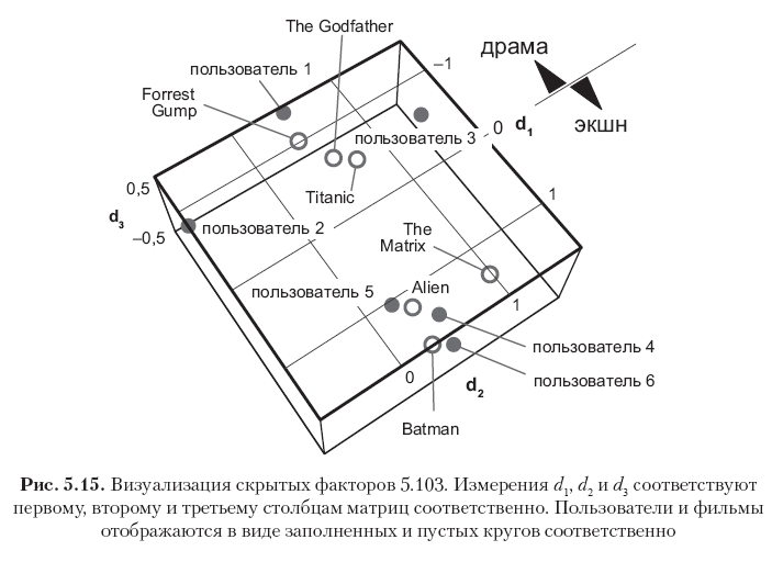
The resulting factor matrices are not completely orthogonal in the columns, but tend to orthogonality, because this follows from the optimality of the SVD solution. This can be seen by considering the works of PTP and QTQ, which are close to diagonal matrices:


Matrices 5.103 are essentially a predictive model that can be used to evaluate both known and absent ratings. Estimates can be obtained by multiplying two factors and adding back the global average:


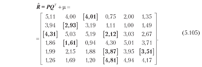
The results accurately reproduce known and predict the missing ratings in accordance with intuitive expectations. The accuracy of the estimates can be increased or decreased by changing the number of measurements, and the optimal number of measurements can be determined in practice by cross-checking and choosing a reasonable compromise between computational complexity and accuracy.

»More information about the book can be found on the publisher's website.
» Table of Contents
» Excerpt

For Habrozhiteley a 25% discount on coupon - Machine Learning

Upon payment of the paper version of the book, an e-book is sent to the e-mail.