Visualization of a column from DataFrame using the library Seaborn
Let's try to visualize the data on advertising campaigns that are stored in the DataFrame.
DataFrame, which stores statistics on advertising campaigns on the following indicators:

')
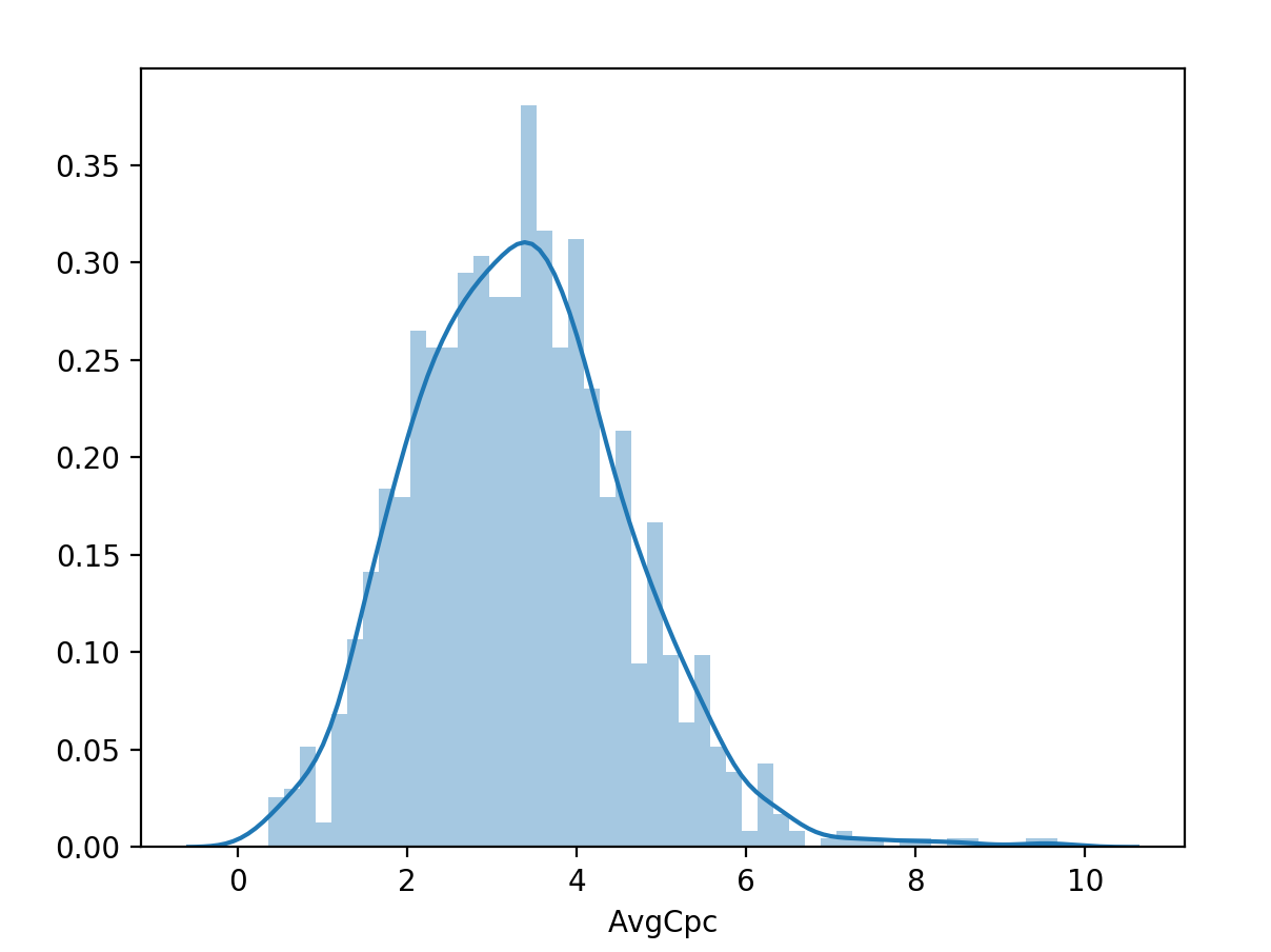
We get the following schedule:

This graph shows the distribution of the cost of clicks. The graph says that most often a click costs about 3.5 rubles.
To make the graph more accurate, you should increase the value in “bins”. This parameter reflects how many parts our chart will be divided into.
We get the following:
You can also replace the histogram with a Rug plot (pad)

Let's return to the histogram.
Color the line blue and the columns blue.

Given:
DataFrame, which stores statistics on advertising campaigns on the following indicators:
- CampaignName
- Date
- Impressions
- Crisks
- Ctr
- Cost
- Avgcpc
- BounceRate
- AvgPageviews
- Conversionsionate
- CostPerConversion
- Conversions
We import everything you need:
import seaborn as sns from pandas import Series,DataFrame Read our DataFrame from csv
f=DataFrame.from_csv("cashe.csv",header=0,sep='',index_col=0,parse_dates=True) ')
Visualize the AvgCpc column data.
sns.distplot(f['AvgCpc'],bins=25) plt.show() We get the following schedule:
This graph shows the distribution of the cost of clicks. The graph says that most often a click costs about 3.5 rubles.
To make the graph more accurate, you should increase the value in “bins”. This parameter reflects how many parts our chart will be divided into.
sns.distplot(f['AvgCpc'],bins=50) plt.show() We get the following:
You can also replace the histogram with a Rug plot (pad)
sns.distplot(f['AvgCpc'],bins=25,rug=True,hist=False) plt.show() Let's return to the histogram.
Set the names and colors
Color the line blue and the columns blue.
sns.distplot(f['AvgCpc'],bins=25, kde_kws={'color':'indianred','label':''}, hist_kws={'color':'blue','label':''}) plt.show() Source: https://habr.com/ru/post/459900/
All Articles