Luxor
Today we look at the graphic package for the Julia language, which is called Luxor . This is one of those tools that turn the process of creating vector images into solving logical problems with a concomitant storm of emotions.
Caution! Under the cut 8.5 MB of lightweight images and gifs depicting psychedelic eggs and four-dimensional objects, viewing of which can cause a slight clouding of reason!
Installation
https://julialang.org - download the Julia distribution from the official site. Then, running the interpreter, we enter commands into its console:
using Pkg Pkg.add("Colors") Pkg.add("ColorSchemes") Pkg.add("Luxor") that installs packages for advanced work with colors and Luxor itself.
Possible problems
The main problem of both modern programming in general and open source in particular is that some projects are built on top of others, inheriting all errors, and even generating new ones due to incompatibilities. Like many other packages, Luxor uses other julia packages for its work, which, in turn, are shells of existing solutions.
So, ImageMagick.jl did not want to load and save files. The solution was found on the original page - it turned out he does not like the Cyrillic alphabet in the ways.
Problem number two arose with the Cairo low-level graphics package on Windows 7. I will tackle the solution here:
- We type in the interpreter
]add Gtk- the package will start to be installed for working with gui and most likely it will fall during the build - Next, download gtk + -bundle_3.6.4-20130513_win64
- In the folder with Julia’s packages, everything was set up during the installation, but during the execution of point one, gtk was not completed, so we downloaded the finished version for our machine - we drop the contents of the downloaded archive into the C: \ Users \ User.julia \ packages \ directory WinRPM \ Y9QdZ \ deps \ usr \ x86_64-w64-mingw32 \ sys-root \ mingw (Your path may differ)
- Run julia and enter
]build Gtkand after buildingusing Gtk, and, for greater fidelity, rebuild Luxor:]build Luxor - Restart julia, and we can safely use everything you need:
using Luxor
In case of other problems, we try to find our case.
If you want to try animation
Luxor package creates animation using ffmpeg , provided it is present on your computer. ffmpeg is a cross-platform open-source library for processing video and audio files, a very useful thing (there is a good excursion to Habré ). Install it:
- We download ffmpeg from offsite. In my case, this is a download for windows
- Unpack and set the path to ffmpeg.exe in the Path variable.
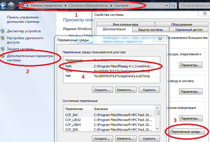
Computer / System Properties / Advanced System Settings / Environment Variables / Path (Create if not) and add the path to your ffmpeg.exe there
Example C: \ Program Files \ ffmpeg-4.1.3-win64-static \ bin
if Path already has values, separate them with a semicolon.
Now, if you enter ffmpeg with the necessary parameters into the command console ( cmd ), it will start and work, and Julia will only communicate with it in this way.
Hello world
Let's start with a small pitfall - when building an image, a graphic file is created and stored in the working directory. That is, when working in the REPL, the julia root folder will be cluttered with pictures, and if you draw in Jupyter, then the pictures are accumulated next to the notepad project, therefore, it will be a good habit to set the working directories in a separate place before starting work:
using Luxor cd("C:\\Users\\User\\Desktop\\mycop") Create the first drawing
Drawing(220, 220, "hw.png") origin() background("white") sethue("black") text("Hello world") circle(Point(0, 0), 100, :stroke) finish() preview() 
Drawing() creates a drawing, in PNG format by default, the default file name is 'luxor-drawing.png', the default size is 800x800, non-integer dimensions can be set for all formats except png, and you can use a sheet of paper ("A0 "," A1 "," A2 "," A3 "," A4 "...)finish() - completes the drawing and closes the file. You can open it in an external viewing application using preview() , which, when working in Jupyter (IJulia), displays the PNG or SVG file in Notepad. When working in Juno, it displays a PNG or SVG file in the Graph panel. In Repl, the image tool that you specified for this format in your OS will be called.
The same can be written in short form using macros.
@png begin text("Hello world") circle(Point(0, 0), 100, :stroke) end For EPS, SVG, PDF vector formats, everything works in a similar way.
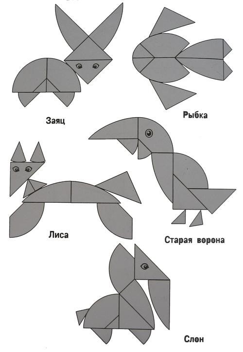
Euclidean egg

This is a rather interesting way of drawing eggs, and if you connect the key points and cut them along the lines, you get a great tangram.
Let's start with the circle:
@png begin radius=80 setdash("dot") sethue("gray30") A, B = [Point(x, 0) for x in [-radius, radius]] line(A, B, :stroke) circle(O, radius, :stroke) end 200 200 "egg0" # 
Everything is very simple: setdash("dot") - draw in dots, sethue("gray30") - color of the line: the smaller, the darker, the closer to 100, the whiter. The point class is defined without us, and the center of coordinates (0,0) can be specified by the letter O Add two circles and sign points:
@png begin radius=80 setdash("dot") sethue("gray30") A, B = [Point(x, 0) for x in [-radius, radius]] line(A, B, :stroke) circle(O, radius, :stroke) label("A", :NW, A) label("O", :N, O) label("B", :NE, B) circle.([A, O, B], 2, :fill) circle.([A, B], 2radius, :stroke) end 600 400 "egg2" 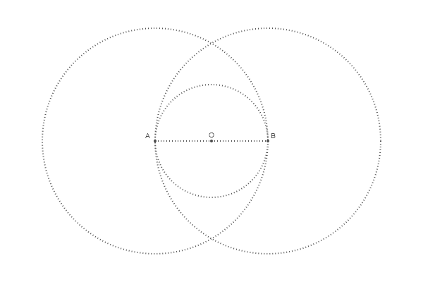
To search for intersection points, there is a function called intersectionlinecircle() that finds the point or points where the line intersects the circle. Thus, we can find two points where one of the circles intersects an imaginary vertical line drawn through O. Because of symmetry, we can only process circle A.
@png begin radius=80 setdash("dot") sethue("gray30") A, B = [Point(x, 0) for x in [-radius, radius]] line(A, B, :stroke) circle(O, radius, :stroke) label("A", :NW, A) label("O", :N, O) label("B", :NE, B) circle.([A, O, B], 2, :fill) circle.([A, B], 2radius, :stroke) # >>>> nints, C, D = intersectionlinecircle(Point(0, -2radius), Point(0, 2radius), A, 2radius) if nints == 2 circle.([C, D], 2, :fill) label.(["D", "C"], :N, [D, C]) end end 600 400 "egg3" 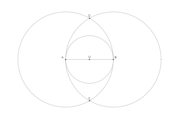
To determine the center of the upper circle we find the intersection OD
@png begin radius=80 setdash("dot") sethue("gray30") A, B = [Point(x, 0) for x in [-radius, radius]] line(A, B, :stroke) circle(O, radius, :stroke) label("A", :NW, A) label("O", :N, O) label("B", :NE, B) circle.([A, O, B], 2, :fill) circle.([A, B], 2radius, :stroke) # >>>> nints, C1, C2 = intersectionlinecircle(O, D, O, radius) if nints == 2 circle(C1, 3, :fill) label("C1", :N, C1) end end 600 400 "egg4" 
The radius of the parenchy circle is determined by the limitation of two large circles:
@png begin radius=80 setdash("dot") sethue("gray30") A, B = [Point(x, 0) for x in [-radius, radius]] line(A, B, :stroke) circle(O, radius, :stroke) label("A", :NW, A) label("O", :N, O) label("B", :NE, B) circle.([A, O, B], 2, :fill) circle.([A, B], 2radius, :stroke) # >>>> nints, C1, C2 = intersectionlinecircle(O, D, O, radius) if nints == 2 circle(C1, 3, :fill) label("C1", :N, C1) end # >>>> nints, I3, I4 = intersectionlinecircle(A, C1, A, 2radius) nints, I1, I2 = intersectionlinecircle(B, C1, B, 2radius) circle.([I1, I2, I3, I4], 2, :fill) # >>>> if distance(C1, I1) < distance(C1, I2) ip1 = I1 else ip1 = I2 end if distance(C1, I3) < distance(C1, I4) ip2 = I3 else ip2 = I4 end label("ip1", :N, ip1) label("ip2", :N, ip2) circle(C1, distance(C1, ip1), :stroke) end 600 400 "egg5" 
Egg is ready! It remains to assemble it from four arcs defined by the arc2r() function and fill the area:
@png begin radius=80 setdash("dot") sethue("gray30") A, B = [Point(x, 0) for x in [-radius, radius]] line(A, B, :stroke) circle(O, radius, :stroke) label("A", :NW, A) label("O", :N, O) label("B", :NE, B) circle.([A, O, B], 2, :fill) circle.([A, B], 2radius, :stroke) # >>>> nints, C1, C2 = intersectionlinecircle(O, D, O, radius) if nints == 2 circle(C1, 3, :fill) label("C1", :N, C1) end # >>>> nints, I3, I4 = intersectionlinecircle(A, C1, A, 2radius) nints, I1, I2 = intersectionlinecircle(B, C1, B, 2radius) circle.([I1, I2, I3, I4], 2, :fill) # >>>> if distance(C1, I1) < distance(C1, I2) ip1 = I1 else ip1 = I2 end if distance(C1, I3) < distance(C1, I4) ip2 = I3 else ip2 = I4 end label("ip1", :N, ip1) label("ip2", :N, ip2) circle(C1, distance(C1, ip1), :stroke) # >>>> setline(5) setdash("solid") arc2r(B, A, ip1, :path) # centered at B, from A to ip1 arc2r(C1, ip1, ip2, :path) arc2r(A, ip2, B, :path) arc2r(O, B, A, :path) strokepreserve() setopacity(0.8) sethue("ivory") fillpath() end 600 400 "egg6" 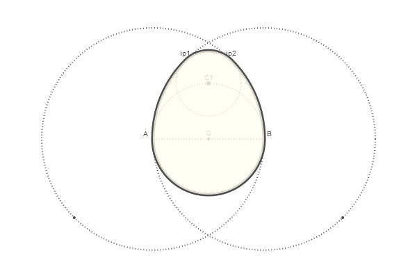
And now, in order to be pampered, we will bring our work in
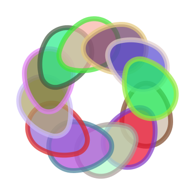
function egg(radius, action=:none) A, B = [Point(x, 0) for x in [-radius, radius]] nints, C, D = intersectionlinecircle(Point(0, -2radius), Point(0, 2radius), A, 2radius) flag, C1 = intersectionlinecircle(C, D, O, radius) nints, I3, I4 = intersectionlinecircle(A, C1, A, 2radius) nints, I1, I2 = intersectionlinecircle(B, C1, B, 2radius) if distance(C1, I1) < distance(C1, I2) ip1 = I1 else ip1 = I2 end if distance(C1, I3) < distance(C1, I4) ip2 = I3 else ip2 = I4 end newpath() arc2r(B, A, ip1, :path) arc2r(C1, ip1, ip2, :path) arc2r(A, ip2, B, :path) arc2r(O, B, A, :path) closepath() do_action(action) end We use random colors, layer drawing and various initial conditions:
@png begin setopacity(0.7) for θ in range(0, step=π/6, length=12) @layer begin rotate(θ) translate(100, 50) # translate(0, -150) #rulers() egg(50, :path) setline(10) randomhue() fillpreserve() randomhue() strokepath() end end end 400 400 "eggs2" 
In addition to strokes and fills, you can use the contour as a clipping region (crop another image into an egg shape) or as a basis for various constructors. The egg () function creates an outline and allows you to apply an action to it. It is also possible to transform our creation into a polygon (an array of points). The following code converts the outline of an egg into a polygon, and then moves every other point of the polygon halfway to the centroid.
@png begin egg(160, :path) pgon = first(pathtopoly()) pc = polycentroid(pgon) circle(pc, 5, :fill) for pt in 1:2:length(pgon) pgon[pt] = between(pc, pgon[pt], 0.5) end poly(pgon, :stroke) end 350 500 "polyegg" 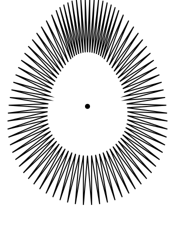
The uneven appearance of the interior points here comes as a result of the default line connection settings. Experiment with setlinejoin("round") to see if this changes the geometry. Now let's try offsetpoly() creating a polygonal contour inside or outside of an existing polygon ..
@png begin egg(80, :path) pgon = first(pathtopoly()) pc = polycentroid(pgon) for pt in 1:2:length(pgon) pgon[pt] = between(pc, pgon[pt], 0.9) end for i in 30:-3:-8 randomhue() op = offsetpoly(pgon, i) poly(op, :stroke, close=true) end end 350 500 "polyeggs" 
Small changes in the regularity of the points created by converting a path to a polygon, and the different number of samples it made, are constantly amplified in successive contours.
Animation
To begin with, let's set functions that implement the background and the drawing of the egg, depending on the frame number:
using Colors demo = Movie(400, 400, "test") function backdrop(scene, framenumber) background("black") end function frame(scene, framenumber) setopacity(0.7) θ = framenumber * π/6 @layer begin rotate(θ) translate(100, 50) egg(50, :path) setline(10) randomhue() fillpreserve() randomhue() strokepath() end end Animation is implemented by a simple set of commands:
animate(demo, [ Scene(demo, backdrop, 0:12), Scene(demo, frame, 0:12, easingfunction=easeinoutcubic, optarg="made with Julia") ], framerate=10, tempdirectory="C:\\Users\\User\\Desktop\\mycop", creategif=true) What actually causes our ffmpeg
run(`ffmpeg -f image2 -i $(tempdirectory)/%10d.png -vf palettegen -y $(seq.stitle)-palette.png`) run(`ffmpeg -framerate 30 -f image2 -i $(tempdirectory)/%10d.png -i $(seq.stitle)-palette.png -lavfi paletteuse -y /tmp/$(seq.stitle).gif`) That is, a series of images is created, and then a gif is assembled from these frames:
Pentachor
He is the fifth book - the correct four-dimensional simplex. In order to draw and manipulate 4-dimensional objects on two-dimensional pictures, first we define
struct Point4D <: AbstractArray{Float64, 1} x::Float64 y::Float64 z::Float64 w::Float64 end Point4D(a::Array{Float64, 1}) = Point4D(a...) Base.size(pt::Point4D) = (4, ) Base.getindex(pt::Point4D, i) = [pt.x, pt.y, pt.z, pt.w][i] struct Point3D <: AbstractArray{Float64, 1} x::Float64 y::Float64 z::Float64 end Base.size(pt::Point3D) = (3, ) Instead of defining a set of operations manually, we can define our structure as a subtype of AbstractArray ( More about classes as interfaces )
The main task we have to solve is how to convert a 4D point to a 2D point. Let's start with a simpler task: how to convert a 3D point to a 2D point, i.e. how can we draw a 3d shape on a flat surface? Consider a simple cube. The front and back surfaces can have the same X and Y coordinates and change only in their Z values.
@png begin fontface("Menlo") fontsize(8) setblend(blend( boxtopcenter(BoundingBox()), boxmiddlecenter(BoundingBox()), "skyblue", "white")) box(boxtopleft(BoundingBox()), boxmiddleright(BoundingBox()), :fill) setblend(blend( boxmiddlecenter(BoundingBox()), boxbottomcenter(BoundingBox()), "grey95", "grey45" )) box(boxmiddleleft(BoundingBox()), boxbottomright(BoundingBox()), :fill) sethue("black") setline(2) bx1 = box(O, 250, 250, vertices=true) poly(bx1, :stroke, close=true) label.(["-1 1 1", "-1 -1 1", "1 -1 1", "1 1 1"], slope.(O, bx1), bx1) setline(1) bx2 = box(O, 150, 150, vertices=true) poly(bx2, :stroke, close=true) label.(["-1 1 0", "-1 -1 0", "1 -1 0", "1 1 0"], slope.(O, bx2), bx2, offset=-45) map((x, y) -> line(x, y, :stroke), bx1, bx2) end 400 400 "cube.png" 
Therefore, the idea is to project a cube from 3D to 2D, saving the first two values and multiplying or changing them to a third value. Check
const K = 4.0 function convert(Point, pt3::Point3D) k = 1/(K - pt3.z) return Point(pt3.x * k, pt3.y * k) end @png begin cube = Point3D[ Point3D(-1, -1, 1), Point3D(-1, 1, 1), Point3D( 1, -1, 1), Point3D( 1, 1, 1), Point3D(-1, -1, -1), Point3D(-1, 1, -1), Point3D( 1, -1, -1), Point3D( 1, 1, -1), ] circle.(convert.(Point, cube) * 300, 5, :fill) end 220 220 "points" 
Using the same principle, let's create a method for converting 4D-points and a function that takes a list of four-dimensional points and displays them twice into a list of two-dimensional points suitable for drawing.
function convert(Point3D, pt4::Point4D) k = 1/(K - pt4.w) return Point3D(pt4.x * k, pt4.y * k, pt4.z * k) end function flatten(shape4) return map(pt3 -> convert(Point, pt3), map(pt4 -> convert(Point3D, pt4), shape4)) end Next, set the vertices and faces and check how it works in color
const n = -1/√5 const pentachoron = [Point4D(vertex...) for vertex in [ [ 1.0, 1.0, 1.0, n], [ 1.0, -1.0, -1.0, n], [-1.0, 1.0, -1.0, n], [-1.0, -1.0, 1.0, n], [ 0.0, 0.0, 0.0, n + √5]]]; const pentachoronfaces = [ [1, 2, 3], [1, 2, 4], [1, 2, 5], [1, 3, 4], [1, 3, 5], [1, 4, 5], [2, 3, 4], [2, 3, 5], [2, 4, 5], [3, 4, 5]]; @png begin setopacity(0.2) pentachoron2D = flatten(pentachoron) for (n, face) in enumerate(pentachoronfaces) randomhue() poly(1500 * pentachoron2D[face], :fillpreserve, close=true) sethue("black") strokepath() end end 300 250 "5ceil" 
Every self-respecting game developer should know the mathematical foundations of computer graphics . If you have never tried to compress, rotate, reflect the teapots in OpenGL - do not worry, it's pretty simple. To reflect a point about a straight line, or to rotate a plane around a certain axis, you need to multiply the coordinates by a special matrix. Actually, we further define the transformation matrices we need:
function XY(θ) [cos(θ) -sin(θ) 0 0; sin(θ) cos(θ) 0 0; 0 0 1 0; 0 0 0 1] end function XW(θ) [cos(θ) 0 0 -sin(θ); 0 1 0 0; 0 0 1 0; sin(θ) 0 0 cos(θ)] end function XZ(θ) [cos(θ) 0 -sin(θ) 0; 0 1 0 0; sin(θ) 0 cos(θ) 0; 0 0 0 1] end function YZ(θ) [1 0 0 0; 0 cos(θ) -sin(θ) 0; 0 sin(θ) cos(θ) 0; 0 0 0 1] end function YW(θ) [1 0 0 0; 0 cos(θ) 0 -sin(θ); 0 0 1 0; 0 sin(θ) 0 cos(θ)] end function ZW(θ) [1 0 0 0; 0 1 0 0; 0 0 cos(θ) -sin(θ); 0 0 sin(θ) cos(θ)]; end function rotate4(A, matrixfunction) return map(A) do pt4 Point4D(matrixfunction * pt4) end end Usually you rotate points on a plane relative to a one-dimensional object. 3D points are around a 2D line (often this is one of the XYZ axes). Thus, it is logical that the 4D points rotate relative to the 3D plane. We defined matrices that perform four-dimensional rotation about the plane defined by the two axes X, Y, Z, and W. The XY plane is usually the plane of the drawing surface. If you perceive the XY plane as a computer screen, the XZ plane is parallel to your desk or floor, and the YZ plane is the wall next to your desk to the right or left. What about XW, YW and ZW? This is the secret of four-dimensional figures: we cannot see these planes, we can only imagine their existence by observing how the forms move through them and around them.
Now we set the functions for the frames and sew the animation:
using ColorSchemes function frame(scene, framenumber, scalefactor=1000) background("white") # antiquewhite setlinejoin("bevel") setline(1.0) sethue("black") eased_n = scene.easingfunction(framenumber, 0, 1, scene.framerange.stop) pentachoron′ = rotate4(pentachoron, XZ(eased_n * 2π)) pentachoron2D = flatten(pentachoron′) setopacity(0.2) for (n, face) in enumerate(pentachoronfaces) sethue(get(ColorSchemes.diverging_rainbow_bgymr_45_85_c67_n256, n/length(pentachoronfaces))) poly(scalefactor * pentachoron2D[face], :fillpreserve, close=true) sethue("black") strokepath() end end function makemovie(w, h, fname; scalefactor=1000) movie1 = Movie(w, h, "4D movie") animate(movie1, Scene(movie1, (s, f) -> frame(s, f, scalefactor), 1:300, easingfunction=easeinoutsine), #framerate=10, tempdirectory="C:\\Users\\User\\Desktop\\mycop", creategif=true, pathname="C:\\Users\\User\\Desktop\\mycop\\$(fname)") end makemovie(320, 320, "pentachoron-xz.gif", scalefactor=2000) 
Well, and another view:
function frame(scene, framenumber, scalefactor=1000) background("antiquewhite") setlinejoin("bevel") setline(1.0) setopacity(0.2) eased_n = scene.easingfunction(framenumber, 0, 1, scene.framerange.stop) pentachoron2D = flatten( rotate4( pentachoron, XZ(eased_n * 2π) * YW(eased_n * 2π))) for (n, face) in enumerate(pentachoronfaces) sethue(get(ColorSchemes.diverging_rainbow_bgymr_45_85_c67_n256, n/length(pentachoronfaces))) poly(scalefactor * pentachoron2D[face], :fillpreserve, close=true) sethue("black") strokepath() end end makemovie(500, 500, "pentachoron-xz-yw.gif", scalefactor=2000) 
Made naturally desire to implement a more popular four-dimensional object - Tesseract
const tesseract = [Point4D(vertex...) for vertex in [ [-1, -1, -1, 1], [ 1, -1, -1, 1], [ 1, 1, -1, 1], [-1, 1, -1, 1], [-1, -1, 1, 1], [ 1, -1, 1, 1], [ 1, 1, 1, 1], [-1, 1, 1, 1], [-1, -1, -1, -1], [ 1, -1, -1, -1], [ 1, 1, -1, -1], [-1, 1, -1, -1], [-1, -1, 1, -1], [ 1, -1, 1, -1], [ 1, 1, 1, -1], [-1, 1, 1, -1]]] const tesseractfaces = [ [1, 2, 3, 4], [1, 2, 10, 9], [1, 4, 8, 5], [1, 5, 6, 2], [1, 9, 12, 4], [2, 3, 11, 10], [2, 3, 7, 6], [3, 4, 8, 7], [5, 6, 14, 13], [5, 6, 7, 8], [5, 8, 16, 13], [6, 7, 15, 14], [7, 8, 16, 15], [9, 10, 11, 12], [9, 10, 14, 13], [9, 13, 16, 12], [10, 11, 15, 14], [13, 14, 15, 16]]; function frame(scene, framenumber, scalefactor=1000) background("black") setlinejoin("bevel") setline(10.0) setopacity(0.7) eased_n = scene.easingfunction(framenumber, 0, 1, scene.framerange.stop) tesseract2D = flatten( rotate4( tesseract, XZ(eased_n * 2π) * YW(eased_n * 2π))) for (n, face) in enumerate(tesseractfaces) sethue([Luxor.lighter_blue, Luxor.lighter_green, Luxor.lighter_purple, Luxor.lighter_red][mod1(n, 4)]...) poly(scalefactor * tesseract2D[face], :fillpreserve, close=true) sethue([Luxor.darker_blue, Luxor.darker_green, Luxor.darker_purple, Luxor.darker_red][mod1(n, 4)]...) strokepath() end end makemovie(500, 500, "tesseract-xz-yw.gif", scalefactor=1000) 
Homework: automate the creation of arrays of coordinates and vertex numbers ( permutations with repetitions and without repetitions, respectively ). We also did not use all the broadcast matrices; Each new perspective causes a new “Wow!”, but I decided not to overload the page. Well, you can experiment with a large number of faces and dimensions.
Links
- Luxor - page on githab
- Luxor docs - a guide with examples
- Cairo - low-level graphics library; used by Luxor as an environment
- The library's author's blog - there are a lot of different styles and more extended examples, including four-dimensional figures.

')
Source: https://habr.com/ru/post/459842/
All Articles