Neural Networks and Deep Learning, Chapter 3, Part 2: Why does regularization help reduce retraining?

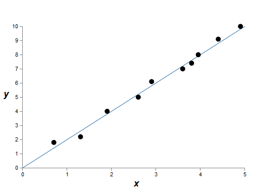
Empirically, we saw that regularization helps reduce retraining. It is inspiring - but, unfortunately, it is not obvious why regularization helps. Usually people explain it this way: in some sense, smaller weights have less complexity, which provides a simpler and more effective explanation of the data, so they should be preferred. However, this is too brief an explanation, and some parts of it may seem dubious or mysterious. Let's expand this story and examine it with a critical eye. To do this, suppose we have a simple data set for which we want to create a model:


By meaning, here we study the phenomenon of the real world, and x and y denote real data. Our goal is to build a model that allows us to predict y as a function of x. We could try to use the neural network to create such a model, but I offer something simpler: I will try to model y as a polynomial from x. I will do this instead of neural networks, since the use of polynomials makes the explanation particularly understandable. As soon as we deal with the case of a polynomial, we turn to the NA. There are ten points on the graph above, which means that we can find a unique 9th order polynomial y = a ₀ x ⁹ + a ₁ x ⁸ + ... + a ₉ that exactly fits the data. And here is the graph of this polynomial.


Perfect hit. But we can get a good approximation using the linear model y = 2x
')

Which one is better? Which one is more likely to be true? Which would be better summarized to other examples of the same phenomenon of the real world?

Difficult questions. And one cannot get accurate answers to them without having additional information about the underlying real-world phenomenon. However, let's consider two possibilities: (1) a model with a 9th order polynomial truly describes the phenomenon of the real world, and therefore, it is generalized perfectly; (2) the correct model is y = 2x, but we have additional noise associated with measurement errors, so the model is not ideal.

A priori, one cannot say which of the two possibilities is correct (or that there is no third one). Logically, any of them may be true. And the difference between them is not trivial. Yes, based on the available data, it can be said that there is only a small difference between the models. But suppose we want to predict the value of y, corresponding to some large value of x, much larger than any of those shown in the graph. If we try to do this, then there will be a huge difference between the predictions of the two models, since the 9th order polynomial is dominated by the term x9, and the linear model remains linear.

One point of view on what is happening is to state that a simpler explanation should be used in science, if possible. When we find a simple model that explains many anchor points, we just want to shout: "Eureka!". After all, it is unlikely that a simple explanation will appear purely by chance. We suspect that the model should give some truth related to the phenomenon. In this case, the model y = 2x + noise seems much simpler than y = a ₀ x ⁹ + a ₁ x ⁸ + ... It would be surprising if simplicity arose by chance, so we suspect that y = 2x + noise expresses some underlying truth. From this point of view, the 9th order model simply studies the effect of local noise. And although the 9th order model works ideally for these specific reference points, it will not be able to generalize to other points, with the result that the predictive capabilities of the linear model with noise will be better.

Let's see what this view means for neural networks. Suppose that in our network there are mostly small weights, as is usually the case in regularized networks. Due to the small weights, the network behavior does not change much when several random inputs change here and there. As a result, a regularized network is difficult to learn the effects of local noise present in the data. This is similar to the desire to ensure that individual evidence does not greatly affect the output of the network as a whole. The regularized network is instead trained to respond to such evidence, which is often found in training data. Conversely, a network with large weights can quite change its behavior in response to small changes in input data. Therefore, an unregularized network can use large weights to train a complex model containing a lot of information about the noise in the training data. In short, the limitations of regularized networks allow them to create relatively simple models based on patterns that are often found in training data, and they are resistant to deviations caused by noise in training data. It is hoped that this will force our networks to study the phenomenon itself, and it is better to generalize the knowledge gained.

Given all this, the idea of ​​giving preference to simpler explanations should make you nervous. Sometimes people call this idea “Occam's razor” and zealously apply it, as if it has the status of a common scientific principle. But this, of course, is not a general scientific principle. There is no a priori logical reason for preferring simple explanations to complex ones. Sometimes a more complicated explanation is correct.

Let me describe two examples of how a more complex explanation turned out to be correct. In the 1940s, physicist Marcel Shane announced the discovery of a new particle. The company he worked for, General Electric, was delighted and widely published this event. However, physicist Hans Bethe was skeptical. Bete visited Shane and studied the plates with traces of Shane's new particle. Shane showed Bete a record after a record, but on each of them, Bethe found some problem that spoke of the need to reject this data. Finally, Shane showed Beta a record that looked fit. Bethe said that this is probably just a statistical deviation. Shane: “Yes, but the chances that this is due to statistics, even by your own formula, are one to five.” Bethe: "However, I have already looked at five records." Finally, Shane said: “But you explained my every plate, every good image by some other theory, and I have one hypothesis explaining all the plates at once, from which it follows that we are talking about a new particle.” Bethe replied: “The only difference between my and your explanations is that yours are wrong, and mys are right. Your single explanation is wrong, but all my explanations are correct. " Subsequently, it turned out that nature agreed with Bethe, and Shane’s particle evaporated.

In the second example, in 1859, the astronomer Urben Jean Joseph Le Verrier discovered that the shape of the orbit of Mercury does not correspond to the theory of the world-wide Newton. There was a tiny deviation from this theory, and then several solutions were proposed to solve the problem, which boiled down to the fact that Newton's theory as a whole is correct, and requires only a small change. And in 1916, Einstein showed that this deviation can be well explained using his general theory of relativity, which is radically different from Newtonian gravity and based on much more complex mathematics. Despite this additional complexity, today it is considered that Einstein's explanation is correct, and Newtonian gravity is incorrect even in a modified form . This happens, in particular, because today we know that Einstein's theory explains many other phenomena with which Newton's theory had difficulties. Moreover, what is even more striking, Einstein's theory accurately predicts several phenomena that Newtonian gravity did not predict at all. However, these impressive qualities were not obvious in the past. If judged on the basis of simplicity alone, then some modified form of Newtonian theory would look more attractive.

Three morals can be learned from these stories. First, it is sometimes quite difficult to decide which of the two explanations will be “easier”. Secondly, even if we made such a decision, simplicity must be guided extremely carefully! Third, the true test of the model is not simplicity, but how well it predicts new phenomena in the new conditions of behavior.

Taking all this into account and being careful, let us take an empirical fact — regularized NAs usually generalize better than non-regularized ones. Therefore, later in the book we will often use regularization. The stories mentioned are only needed to explain why no one has yet developed a fully convincing theoretical explanation for why regularization helps networks to generalize. Researchers continue to publish papers where they try to try different approaches to regularization, compare them, depending on what works best, and try to understand why different approaches work worse or better. So regularization can be treated as a kluj . When it quite often helps, we do not have a completely satisfactory systematic understanding of what is happening - only incomplete heuristic and practical rules.

Here lies a deeper set of problems going to the very heart of science. This is a question of generalization. Regularization can give us a computational magic wand that helps our networks better summarize the data, but does not give a basic understanding of how the generalization works, and what is the best approach to it.

These problems go back to the problem of induction , the famous understanding of which was conducted by the Scottish philosopher David Hume in the book Research on Human Knowledge (1748). The induction problem is devoted to the “ absence of free lunch theorem ” by David Walpert and William Macready (1977).

This is especially annoying, because in ordinary life people are phenomenally well able to summarize data. Show some pictures of an elephant to a child, and he will quickly learn to recognize other elephants. Of course, he can sometimes be mistaken, for example, confuse a rhino with an elephant, but in general this process works surprisingly accurately. Here, we have a system - the human brain - with a huge number of free parameters. And after being shown one or more training images, the system learns to generalize them to other images. Our brain, in a sense, is remarkably well regularized! But how do we do it? At the moment we do not know. I think that in the future we will develop more powerful regularization technologies in artificial neural networks, techniques that ultimately allow the National Assembly to compile data based on even smaller data sets.

In fact, our networks already generalize much better than one could expect a priori. A network with 100 hidden neurons has almost 80,000 parameters. We have only 50,000 images in the training data. It is all the same as trying to pull a polynomial of 80,000 orders of magnitude on 50,000 reference points. By all indications, our network must be terribly retrained. And yet, as we have seen, such a network actually summarizes quite well. Why it happens? This is not entirely clear. It was hypothesized that “the dynamics of learning by gradient descent in multilayer networks is subject to self-regularization”. This is an extraordinary success, but also a rather alarming fact, since we do not understand why this is happening. In the meantime, we will adopt a pragmatic approach, and we will use regularization wherever possible. This will benefit our NA.

Let me finish this section by returning to what I have not explained before: that the L2 regularization does not limit the bias. Naturally, it would be easy to change the regularization procedure so that it regularizes the displacements. But empirically, this often does not change the results in any noticeable way; therefore, to some extent, it is a matter of agreement to engage in regularization of biases. However, it is worth noting that a large offset does not make a neuron sensitive to inputs, like large weights. Therefore, we do not need to worry about large biases that allow our networks to learn noise in the training data. At the same time, by allowing large displacements, we make our networks more flexible in their behavior — in particular, large displacements facilitate the saturation of neurons, which we would like. For this reason, we usually do not include offsets in the regularization.

Other regularization techniques

There are many regularization techniques besides L2. In fact, so many technicians have already been developed that I would not have been able to briefly describe them all with all my desire. In this section, I will briefly describe three other approaches to reducing retraining: L1 regularization, the [dropout] exception , and the artificial increase in the training set. We will not study them as deeply as previous topics. Instead, we will simply get to know them, and at the same time we will evaluate the variety of existing regularization techniques.

L1 Regularization

In this approach, we change the unregularized cost function by adding the sum of the absolute values ​​of the weights:

$$

$$C = C_0 + \ frac {\ lambda} {n} \ sum_w | w | \ tag {95}$$

Intuitively, this is similar to the L2 regularization, which penalizes large weights and makes the network prefer small weights. Of course, the regularization term L1 is not similar to the regularization term L2, so you should not expect exactly the same behavior. Let's try to understand what the behavior of a network trained with L1 regularization differs from a network trained with L2 regularization.

To do this, look at the partial derivatives of the cost function. Differentiating (95), we get:

$$

$$\ frac {\ partial C} {\ partial w} = \ frac {\ partial C_0} {\ partial w} + \ frac {\ lambda} {n} \, {\ rm sgn} (w) \ tag {96 }$$

where sgn (w) is the sign of w, that is, +1 if w is positive, and -1 if w is negative. Using this expression, we modify the backward propagation so that it performs a stochastic gradient descent using L1 regularization. Final update rule for L1-regularized network:

$$

$$w \ rightarrow w '= w- \ frac {\ eta \ lambda} {n} \ mbox {sgn} (w) - \ eta \ frac {\ partial C_0} {\ partial w} \ tag {97}$$

where, as usual, ∂C / ∂w can be optionally estimated through the average value of the mini-package. Let us compare this with the rule for updating the regularization of L2 (93):

$$

$$w \ rightarrow w '= w \ left (1 - \ frac {\ eta \ lambda} {n} \ right) - \ eta \ frac {\ partial C_0} {\ partial w} \ tag {98}$$

In both expressions, the effect of regularization is to reduce weights. This coincides with the intuitive notion that both types of regularization penalize large weights. However, weight is reduced in different ways. In the regularization of L1, the weights are reduced by a constant value, tending to 0. In the regularization of L2, the weights are reduced by a value proportional to w. Therefore, when some weight has a large value of | w |, the regularization of L1 reduces the weight not so much as L2. Conversely, when | w | little, the regularization of L1 reduces the weight much more than the regularization of L2. As a result, the L1 regularization tends to concentrate the weights of the network in a relatively small number of links of high importance, while other weights tend to zero.

I slightly smoothed one problem in the previous discussion - the partial derivative C / ∂w is not defined when w = 0. This is because the function | w | there is a sharp “break” at the point w = 0, therefore it cannot be differentiated there. But it's not scary. We simply apply the usual, non-regularized rule for stochastic gradient descent when w = 0. Intuitively, there is nothing bad in this — regularization should reduce weights, and obviously it cannot reduce a weight already equal to 0. More precisely, we will use equations (96) and (97) with the condition that sgn (0) = 0 This will give us a convenient and compact rule for stochastic gradient descent with L1 regularization.

Exception [dropout]

The exception is a completely different regularization technique. In contrast to the regularization of L1 and L2, the exception does not deal with the change in the cost function. Instead, we change the network itself. Let me explain the basic mechanics of the exception, before delving into the topic of why it works and with what results.

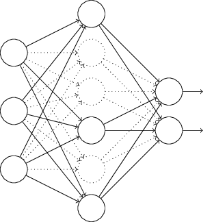
Suppose we are trying to train the network:


In particular, let's say we have training input x and the corresponding desired output y. Usually we would train it by direct propagation x over the network, and then back propagation to determine the gradient contribution. An exception alters this process. We begin with the random and temporary removal of half of the hidden neurons of the network, leaving the input and output neurons unchanged. After that, we will have about such a network. Note that the excluded neurons, those that are temporarily removed, are still marked on the diagram:


We transmit x by direct distribution through the modified network, and then we distribute the result back, also through the modified network. After we do this with a mini-package of examples, we update the corresponding weights and offsets. Then we repeat this process, first restoring the excluded neurons, then selecting a new random subset of hidden neurons to remove, evaluating the gradient for another mini-packet, and updating the network weights and offsets.

Repeating this process over and over again, we get a network that has learned some weights and offsets. Naturally, these weights and displacements were learned under conditions in which half of the hidden neurons were excluded. And when we launch the network to its fullest, we will have twice as many active hidden neurons. In order to compensate for this, we are balancing the weights emanating from hidden neurons.

The exclusion procedure may seem strange and arbitrary. Why should she help with regularization? To explain what is happening, I want you to forget about the exception for a while, and to present the NA training in a standard way. In particular, imagine that we train several different NSs using the same training data. Of course, the networks may differ at first, and sometimes the training may produce different results. In such cases, we could apply some kind of averaging or voting scheme to decide which one to take. For example, if we trained five networks, and three of them classify a digit as “3,” then it’s probably a triple. And the other two networks are probably just wrong. Such an averaging scheme often proves to be a useful (albeit expensive) way to reduce retraining. The reason is that different networks can be retrained in different ways, and averaging can help with the elimination of such retraining.

How does all this relate to the exception? Heuristically, when we exclude different sets of neutrons, it is as if we were teaching different NSs. Therefore, the exclusion procedure is similar to averaging effects over a very large number of different networks. Different networks retrain differently, so there is hope that the average exclusion effect will reduce retraining.

A related heuristic explanation of the benefits of exclusion is given in one of the earliest works that used this technique: “This technique reduces the complex joint adaptation of neurons, since a neuron cannot rely on the presence of certain neighbors. As a result, he has to learn more reliable features that can be useful in working with many different random subsets of neurons. ” In other words, if we present our NA as a model that makes predictions, the exception would be a way to guarantee the stability of the model to the loss of certain parts of evidence. In this sense, the technique resembles the regularizations of L1 and L2, seeking to reduce weights, and thus making the network more resistant to the loss of any individual connections in the network.

Naturally, the true measure of the utility of an exception is its tremendous success in improving the efficiency of neural networks. In the original workwhere this method was presented, it was applied to many different tasks. We are particularly interested in the fact that the authors applied an exception to the classification of numbers from MNIST, using a simple direct distribution network, similar to the one we considered. The paper notes that until then, the best result for such an architecture was 98.4% accuracy. They improved it to 98.7% using a combination of elimination and a modified form of the regularization of L2. Similarly impressive results were obtained for many other tasks, including pattern and speech recognition, and natural language processing. The exception was especially useful in training large deep networks, where the problem of retraining often arises.

Artificial extension of the training data set

Earlier, we saw that our MNIST classification accuracy dropped to 80 percent with something when we used only 1,000 training images. And no wonder - with less data, our network will meet fewer options for writing numbers with people. Let's try to train our network of 30 hidden neurons using different volumes of the training set to look at the change in efficiency. We train using the mini package size of 10, the learning rate is η = 0.5, the regularization parameter is λ = 5.0, and the cost function with cross entropy. We will train a network of 30 epochs using the full set of data, and increase the number of epochs in proportion to the reduction in the amount of training data. To ensure the same weight reduction factor for different sets of training data, we will use the regularization parameter λ = 5,0 with a full training set, and proportionally reduce it with decreasing data volumes.


It can be seen that the classification accuracy increases significantly with the increase in the volume of training data. Probably, this growth will continue with a further increase in volumes. Of course, judging by the graph above, we are approaching saturation. However, suppose that we redo this graph into a logarithmic dependence on the amount of training data:


It is seen that at the end of the schedule still tends up. This suggests that if we take a much more massive amount of data — say, millions or even billions of handwritten examples, rather than 50,000 — then we will probably get a much better working network of even such a small size.

Getting more tutorial data is a great idea. Unfortunately, this can be expensive, so in practice it is not always possible. However, there is another idea that can work almost as well - to artificially increase the data set. For example, let's say we take an image of the five from MNIST, and rotate it a little, by 15 degrees:



This is clearly the same figure. But at the pixel level, it is very different from the images available in the MNIST database. It is reasonable to assume that adding this image to a training data set can help our network learn more about image classification. Moreover, we are obviously not limited to the possibility of adding just one image. We can expand our training data by making a few small turns of all the training pictures from MNIST, and then using the extended set of training data to increase the efficiency of the network.

This idea is very powerful, and it is widely used. Let's look at the results from scientific workwhich applied several variations of this idea to MNIST. One of the architectures of the networks under consideration was similar to the one we are using - a network with direct propagation with 800 hidden neurons, using the cost function with cross-entropy. By launching this network with the standard MNIST training set, they obtained a classification accuracy of 98.4%. But then they expanded the training data, using not only the rotation I described above, but also the transfer and distortion of images. Having trained the network on extended data, they increased its accuracy to 98.9%. They also experimented with the so-called. "Elastic distortion", a special type of image distortion, designed to eliminate random fluctuations of the muscles of the hand. Using elastic distortion to expand the data, they achieved an accuracy of 99.3%. In fact, they extended the experience of their network,giving her various handwriting variations found in real handwriting.

Variants of this idea can be used to improve the performance of a multitude of learning tasks, not only for handwriting recognition. The general principle is to expand the training data by applying to it operations that reflect the variations encountered in reality. Such variations are easy to come up with. Suppose we create a speech recognition language. People can recognize speech even if there are distortions such as background noise. Therefore, you can expand the data by adding background noise. We are also able to recognize accelerated and slow speech. This is another way to expand the training data. These techniques are not always used — for example, instead of expanding the training set through adding noise, it may be more efficient to clean up the input data by applying a noise filter to them. And yet, it is worth bearing in mind the idea of ​​expanding the training set,and look for ways to apply it.

Exercise

• As we discussed above, one of the ways to expand the learning data from MNIST is to use small turns of the training pictures. What problem may arise if we allow the rotation of pictures at any angles?

Big Data Deviation and the Meaning of Comparing Classification Accuracy

Let's look again at how the accuracy of our NA varies with the size of the training set:


Suppose that instead of using NA, we would use another machine learning technology to classify numbers. For example, we will try to use the support vector machine (support vector machine, SVM) method, which we briefly met in Chapter 1. As then, do not worry if you are not familiar with SVM, we do not need to understand its details. We will use SVM at the expense of the scikit-learn library. This is how the effectiveness of the SVM varies depending on the size of the training set. For comparison, I put on the schedule and the results of the NA.


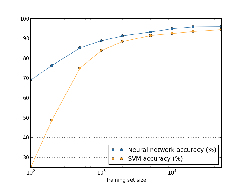
Probably the first thing that catches the eye - NA exceeds the SVM on any size of the training set. This is good, although you should not make far-reaching conclusions from this, since I used the scikit-learn pre-installed settings, and we worked quite seriously on our NA. A less vivid, but more interesting fact, which follows from the graph, is that if we train our SVM using 50,000 images, it will work better (accuracy 94.48%) than our NS trained in 5000 images ( 93.24%). In other words, an increase in the amount of training data sometimes compensates for the difference in MO algorithms.

Something more interesting might happen. Suppose we are trying to solve a problem using two algorithms MO, A and B. Sometimes it happens that algorithm A is ahead of algorithm B on one set of training data, and algorithm B is ahead of algorithm A on another set of training data. Above, we did not see this - then the graphics would have crossed - but it happens . The correct answer to the question: “Does algorithm A surpass algorithm B?” Is actually this: “What training data set do you use?”

All this must be taken into account, both during development and during the reading of scientific papers. Many papers concentrate on finding new tricks for squeezing the best results on standard measurement data sets. “Our super-duper technology gave us an X% improvement on the standard comparative set Y” is the canonical form of the statement in such a study. Sometimes such statements are actually interesting, but it is worth understanding that they are applicable only in the context of a specific training set. Imagine an alternative story in which people who initially created a comparative set received a larger research grant. They could use extra money to collect additional data. It is possible that the “improvement” of the super-duper technology would disappear on a larger data set. In other words,The essence of the improvement may be just an accident. From this to the area of ​​practical application, we need to take the following morality: we need both an improvement of the algorithms and an improvement in the training data. There is nothing wrong with looking for improved algorithms, but make sure that you are not concentrating on this, ignoring an easier way to win by increasing the amount or quality of the training data.

Task

• . ? . – , , , . , . - ? , .

Results

We have completed our immersion in retraining and regularization. We, of course, will return to these problems. As I have mentioned several times, retraining is a big problem in the field of NA, especially as computers become more powerful and we can train ever larger networks. As a result, there is an urgent need to develop effective regularization techniques to reduce retraining, so this area is very active today.

Scale Initialization

When we create our NA, we need to make a choice of the initial values ​​of weights and displacements. So far we have chosen them according to the prescriptions I briefly described in Chapter 1. Let me remind you that we chose weights and displacements based on an independent Gaussian distribution with a mean of 0 and a standard deviation of 1. This approach worked well, but it seems rather arbitrary, therefore revise it and consider whether it is possible to find the best way to assign initial weights and offsets, and, perhaps, help our NA learn faster.

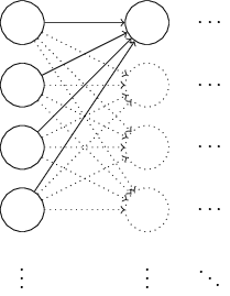
It turns out that you can quite seriously improve the initialization process compared to the normalized Gaussian distribution. To understand this, let's say we work with a network with a large number of input neurons, say, 1000. And suppose we used the normalized Gaussian distribution to initialize weights connected to the first hidden layer. So far, I will focus only on the scales connecting the input neurons to the first neuron in the hidden layer, and ignore the rest of the network:


For simplicity, let us imagine that we are trying to train the network with input x, in which half of the input neurons are turned on, that is, have the value 1, and half are turned off, that is, have the value 0. The following argument works in a more general case, but it's easier for you will understand it on this particular example. Consider the weighted sum Σ = z _j w _j x _j + b inputs to the hidden neuron. 500 member amounts disappear because the corresponding x _jequal to 0. Therefore, z is the sum of 501 normalized Gaussian random variables, 500 weights and 1 additional offset. Therefore, the value of z itself has a Gaussian distribution with a mathematical expectation of 0 and a standard deviation of √ 501 ≈ 22.4. That is, z has a fairly wide Gaussian distribution, without sharp peaks:


In particular, this graph shows that | z | is likely to be quite large, that is, z ≫ 1 or z ≫ -1. In this case, the output of the hidden neurons σ (z) will be very close to 1 or 0. This means that our hidden neuron will be saturated. And when this happens, as we already know, small changes in the weights will produce tiny changes in the activation of the hidden neuron. These tiny changes, in turn, practically do not affect the remaining neutrons in the network, and we will see the corresponding tiny changes in the cost function. As a result, these weights will be learned very slowly when we use the gradient descent algorithm. This is similar to the task we have already discussed in this chapter, in which the output neurons saturated with incorrect values ​​cause learning to slow down. Previously, we solved this problem by cleverly choosing the cost function.Unfortunately, although it helped with saturated output neurons, it does not help at all with saturating hidden neurons.

Now I talked about the incoming scales of the first hidden layer. Naturally, the same arguments apply to the following hidden layers: if the weights in the late hidden layers are initialized using normalized Gaussian distributions, their activation will often be close to 0 or 1, and learning will go very slowly.

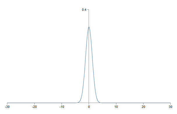
Is there a way to choose the best initialization options for weights and offsets, so that we do not get such saturation, and can avoid slowing down learning? Suppose we have a neuron with the number of incoming scales n _in . Then we need to initialize these weights with random Gaussian distributions with expectation 0 and standard deviation 1 / √n _in. That is, we compress the Gaussians, and reduce the likelihood of saturation of the neuron. Then we will choose a Gaussian distribution for offsets with a mean of 0 and a standard deviation of 1, for reasons I’ll come back to later. Having made this choice, we again obtain that z = ∑ _j w _j x _j+ b will be a random variable with a Gaussian distribution with a mean of 0, but with a much more pronounced peak than before. Suppose, as before, that 500 inputs are 0, and 500 are equal to 1. Then it is easy to show (see the exercise below) that z has a Gaussian distribution with an expectation of 0 and a standard deviation of √ (3/2) = 1.22 ... This graph has a much sharper peak, so much so that even in the picture below, the situation is somewhat understated, since I had to change the scale of the vertical axis compared to the previous graph:


Such a neuron is satiated with a much lower probability, and, accordingly, is less likely to face a slowdown in learning.

Exercise

• , z = ∑ _j w _j x _j + b √(3/2). : ; .

I mentioned above that we will continue to initialize the displacements, as before, on the basis of an independent Gaussian distribution with an expectation of 0 and a standard deviation of 1. And this is normal, since it does not greatly increase the likelihood of saturation of our neurons. In fact, the initialization of the displacements does not matter if we can avoid the problem of saturation. Some even try to initialize all zero shifts, and rely on the fact that gradient descent can learn the appropriate shifts. But since the likelihood that this will affect something is small, we will continue to use the same initialization procedure as before.

Let's compare the results of the old and new approaches to initializing weights using the task of classifying numbers from MNIST. As before, we will use 30 hidden neurons, a mini packet of 10 in size, the regularization parameter l = 5.0, and the cost function with cross-entropy. We will gradually reduce the learning rate from η = 0.5 to 0.1, since this way the results will be slightly better seen in the graphs. You can learn using the old method of initializing the scales:

>>> import mnist_loader >>> training_data, validation_data, test_data = \ ... mnist_loader.load_data_wrapper() >>> import network2 >>> net = network2.Network([784, 30, 10], cost=network2.CrossEntropyCost) >>> net.large_weight_initializer() >>> net.SGD(training_data, 30, 10, 0.1, lmbda = 5.0, ... evaluation_data=validation_data, ... monitor_evaluation_accuracy=True) 

You can also learn using the new approach to initializing weights. This is even simpler, because by default network2 initializes weights using a new approach. This means that we can omit the net.large_weight_initializer () call earlier:

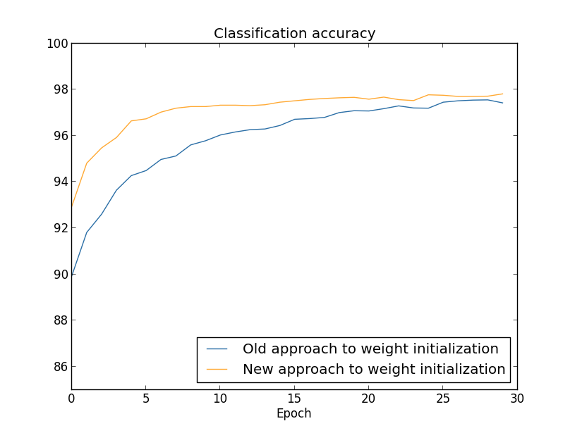
 >>> net = network2.Network([784, 30, 10], cost=network2.CrossEntropyCost) >>> net.SGD(training_data, 30, 10, 0.1, lmbda = 5.0, ... evaluation_data=validation_data, ... monitor_evaluation_accuracy=True) 

Build a graph (using the program weight_initialization.py):


In both cases, a classification accuracy of around 96% is obtained. The final accuracy is almost the same in both cases. But the new initialization technique reaches this point much, much faster. At the end of the last training epoch, the old approach to the initialization of weights reaches an accuracy of 87%, and the new approach is already approaching 93%. Apparently, the new approach to the initialization of the scales begins with a much better position, thanks to which we get good results much faster. The same phenomenon is observed if we construct results for a network with 100 neurons:


In this case, two curves are not found. However, my experiments say that if you add a few more epochs, then the accuracy begins to almost coincide. Therefore, on the basis of these experiments, it can be said that improving the initialization of weights only accelerates learning, but does not change the net effectiveness of the network. However, in Chapter 4 we will see examples of NA, in which the long-term efficiency is greatly improved by the initialization of the scales through 1 / √ n _in . Therefore, not only the learning speed improves, but sometimes the overall effectiveness.

The approach to the initialization of weights through 1 / √n _in helps to improve the training of neural networks. Other techniques for initializing weights have been proposed, many of which are based on this basic idea. I will not consider them here, because for our purposes it works well and 1 / √n _in . If you're interested, I recommend reading the discussion on pages 14 and 15 in the work of 2012 by Joshua Bengio.

Task

• Combining regularization and improved method of initializing weights. Sometimes L2 regularization automatically gives us results similar to the new method of initializing weights. Suppose we use the old approach to initializing weights. Sketch a heuristic argument, proving that: (1) if λ is not too small, then in the first training epochs the weakening of the weights will dominate almost completely; (2) if ηλ ≪ n, then the weights will be weakened by e ^{−ηλ / m} times in the epoch; (3) if λ is not too large, the weakening of the scales will slow down when the weights decrease to a size of about 1 / √ n, where n is the total number of weights in the network. Prove that these conditions are satisfied in the examples for which graphs are constructed in this section.

Back to handwriting recognition: code

Let's implement the ideas described in this chapter. We will develop a new program, network2.py, an improved version of the network.py program we created in Chapter 1. If you haven’t seen its code for a long time, you may need to quickly run through it. This is only 74 lines of code and is easy to understand.

As in the case of network.py, the star of the network2.py program will be the Network class, which we use to represent our national systems. We initialize the class instance with a list of the sizes of the corresponding layers of the network, and the choice of the cost function; by default, this will be the cross entropy:

 class Network(object): def __init__(self, sizes, cost=CrossEntropyCost): self.num_layers = len(sizes) self.sizes = sizes self.default_weight_initializer() self.cost=cost 

The first couple of lines of the __init__ method coincides with network.py, and are self-explanatory. The next two lines are new, and we need to understand in detail what they are doing.

Let's start with the default_weight_initializer method. It uses a new, improved approach to initializing weights. As we have seen, in this approach, the weights entering the neuron are initialized on the basis of an independent Gaussian distribution with a mean of 0 and a standard deviation of 1 divided by the square root of the number of incoming connections to the neuron. Also this method will initialize and offsets using a Gaussian distribution with a mean of 0 and a standard deviation of 1. Here is the code:

  def default_weight_initializer(self): self.biases = [np.random.randn(y, 1) for y in self.sizes[1:]] self.weights = [np.random.randn(y, x)/np.sqrt(x) for x, y in zip(self.sizes[:-1], self.sizes[1:])] 

To understand it, you need to remember that np is the Numpy library that deals with linear algebra. We imported it at the beginning of the program. Also note that we are not initializing offsets in the first layer of neurons. The first layer is incoming, so no offsets are used. The same was network.py.

In addition to the default_weight_initializer method, we will make the method large_weight_initializer. It initializes weights and offsets using the old approach from Chapter 1, where weights and offsets are initialized based on an independent Gaussian distribution with a mean of 0 and a standard deviation of 1. This code, of course, differs little from default_weight_initializer:

  def large_weight_initializer(self): self.biases = [np.random.randn(y, 1) for y in self.sizes[1:]] self.weights = [np.random.randn(y, x) for x, y in zip(self.sizes[:-1], self.sizes[1:])] 

I have included this method mainly because it is more convenient for us to compare the results of this chapter and chapter 1. I cannot imagine any real options in which I would recommend using it!

The second novelty of the __init__ method is the initialization of the cost attribute. To understand how this works, let's look at the class we use to represent the cost function with cross entropy (the @staticmethod directive tells the interpreter that this method does not depend on the object, so the transfer of the self parameter to the fn and delta methods does not occur).

 class CrossEntropyCost(object): @staticmethod def fn(a, y): return np.sum(np.nan_to_num(-y*np.log(a)-(1-y)*np.log(1-a))) @staticmethod def delta(z, a, y): return (ay) 

Let's figure it out. The first thing that can be seen here is that, although from a mathematical point of view, the cross-sectional entropy is a function, we implement it as a python class, and not a python function. Why did I decide to do this? In our network, cost plays two different roles. Obvious - it is a measure of how well the output activation a corresponds to the desired output y. This role is provided by the CrossEntropyCost.fn method. (By the way, we note that calling np.nan_to_num inside CrossEntropyCost.fn ensures that Numpy correctly processes the logarithm of numbers close to zero). However, the cost function is used in our network and in the second way. From Chapter 2, recall that when running the back-propagation algorithm, we need to read the network error δ ^L. The form of the output error depends on the cost function: different cost functions will have different forms of the output error. For cross entropy, the output error, as follows from equation (66), will be equal to:

$$

$$\ delta ^ L = a ^ L-y \ tag {99}$$

Therefore, I define the second method, CrossEntropyCost.delta, whose goal is to explain the networks, how to calculate the output error. And then we combine these two methods into one class, containing everything that our network needs to know about the cost function.

For a similar reason, network2.py contains a class representing a quadratic cost function. Including this for comparison with the results of Chapter 1, since in the future we will mainly use cross entropy. Code below. The QuadraticCost.fn method is a simple calculation of the quadratic cost associated with the output a and the desired output y. The value returned by QuadraticCost.delta is based on expression (30) for the output quadratic cost error, which we derived in Chapter 2.

 class QuadraticCost(object): @staticmethod def fn(a, y): return 0.5*np.linalg.norm(ay)**2 @staticmethod def delta(z, a, y): return (ay) * sigmoid_prime(z) 

Now we understand the main differences between network2.py and network2.py. Everything is very simple. There are other minor changes that I will describe below, including the implementation of the L2 regularization. Before that, let's look at the full network2.py code. It is not necessary to study it in detail, but it is worth understanding the basic structure, in particular, reading the comments in order to understand what each of the program’s pieces does. Of course, I do not forbid to go into this question as much as you like! If you get lost, try reading the text after the program, and return to the code again. So here it is:

 """network2.py ~~~~~~~~~~~~~~   network.py,            .   –      , ,   .     ,    .   ,       . """ ####  #  import json import random import sys #  import numpy as np ####   ,      class QuadraticCost(object): @staticmethod def fn(a, y): """ ,    ``a``    ``y``. """ return 0.5*np.linalg.norm(ay)**2 @staticmethod def delta(z, a, y): """  delta   .""" return (ay) * sigmoid_prime(z) class CrossEntropyCost(object): @staticmethod def fn(a, y): """ ,    ``a``    ``y``. np.nan_to_num    .  ,   ``a``  ``y``      1.0,   (1-y)*np.log(1-a)  nan. np.nan_to_num ,       (0.0). """ return np.sum(np.nan_to_num(-y*np.log(a)-(1-y)*np.log(1-a))) @staticmethod def delta(z, a, y): """  delta   .  ``z``    ,          delta     . """ return (ay) ####   Network class Network(object): def __init__(self, sizes, cost=CrossEntropyCost): """  sizes      .  ,      Network      ,     ,     ,    ,  [2, 3, 1].       ,   ``self.default_weight_initializer`` (.  ). """ self.num_layers = len(sizes) self.sizes = sizes self.default_weight_initializer() self.cost=cost def default_weight_initializer(self): """            0    1,       ,       .          0    1.    ,         ,           . """ self.biases = [np.random.randn(y, 1) for y in self.sizes[1:]] self.weights = [np.random.randn(y, x)/np.sqrt(x) for x, y in zip(self.sizes[:-1], self.sizes[1:])] def large_weight_initializer(self): """          0    1.          0    1.    ,         ,           .         1,    .       . """ self.biases = [np.random.randn(y, 1) for y in self.sizes[1:]] self.weights = [np.random.randn(y, x) for x, y in zip(self.sizes[:-1], self.sizes[1:])] def feedforward(self, a): """  ,  ``a``  .""" for b, w in zip(self.biases, self.weights): a = sigmoid(np.dot(w, a)+b) return a def SGD(self, training_data, epochs, mini_batch_size, eta, lmbda = 0.0, evaluation_data=None, monitor_evaluation_cost=False, monitor_evaluation_accuracy=False, monitor_training_cost=False, monitor_training_accuracy=False): """     -    . ``training_data`` –   ``(x, y)``,       .       ,    ``lmbda``.    ``evaluation_data``,     ,   .         ,     ,   .      :   ,    ,   ,              .  ,      30 ,        30 ,        .     ,   . """ if evaluation_data: n_data = len(evaluation_data) n = len(training_data) evaluation_cost, evaluation_accuracy = [], [] training_cost, training_accuracy = [], [] for j in xrange(epochs): random.shuffle(training_data) mini_batches = [ training_data[k:k+mini_batch_size] for k in xrange(0, n, mini_batch_size)] for mini_batch in mini_batches: self.update_mini_batch( mini_batch, eta, lmbda, len(training_data)) print "Epoch %s training complete" % j if monitor_training_cost: cost = self.total_cost(training_data, lmbda) training_cost.append(cost) print "Cost on training data: {}".format(cost) if monitor_training_accuracy: accuracy = self.accuracy(training_data, convert=True) training_accuracy.append(accuracy) print "Accuracy on training data: {} / {}".format( accuracy, n) if monitor_evaluation_cost: cost = self.total_cost(evaluation_data, lmbda, convert=True) evaluation_cost.append(cost) print "Cost on evaluation data: {}".format(cost) if monitor_evaluation_accuracy: accuracy = self.accuracy(evaluation_data) evaluation_accuracy.append(accuracy) print "Accuracy on evaluation data: {} / {}".format( self.accuracy(evaluation_data), n_data) print return evaluation_cost, evaluation_accuracy, \ training_cost, training_accuracy def update_mini_batch(self, mini_batch, eta, lmbda, n): """    ,          -. ``mini_batch`` –    ``(x, y)``, ``eta`` –  , ``lmbda`` -  , ``n`` -     .""" nabla_b = [np.zeros(b.shape) for b in self.biases] nabla_w = [np.zeros(w.shape) for w in self.weights] for x, y in mini_batch: delta_nabla_b, delta_nabla_w = self.backprop(x, y) nabla_b = [nb+dnb for nb, dnb in zip(nabla_b, delta_nabla_b)] nabla_w = [nw+dnw for nw, dnw in zip(nabla_w, delta_nabla_w)] self.weights = [(1-eta*(lmbda/n))*w-(eta/len(mini_batch))*nw for w, nw in zip(self.weights, nabla_w)] self.biases = [b-(eta/len(mini_batch))*nb for b, nb in zip(self.biases, nabla_b)] def backprop(self, x, y): """  ``(nabla_b, nabla_w)``,      C_x. ``nabla_b``  ``nabla_w`` -    numpy,   ``self.biases`` and ``self.weights``.""" nabla_b = [np.zeros(b.shape) for b in self.biases] nabla_w = [np.zeros(w.shape) for w in self.weights] #   activation = x activations = [x] #      zs = [] #     z- for b, w in zip(self.biases, self.weights): z = np.dot(w, activation)+b zs.append(z) activation = sigmoid(z) activations.append(activation) # backward pass delta = (self.cost).delta(zs[-1], activations[-1], y) nabla_b[-1] = delta nabla_w[-1] = np.dot(delta, activations[-2].transpose()) """  l      ,      . l = 1    , l = 2 – ,   .    ,   python      . """ for l in xrange(2, self.num_layers): z = zs[-l] sp = sigmoid_prime(z) delta = np.dot(self.weights[-l+1].transpose(), delta) * sp nabla_b[-l] = delta nabla_w[-l] = np.dot(delta, activations[-l-1].transpose()) return (nabla_b, nabla_w) def accuracy(self, data, convert=False): """    ``data``,      .   –        .  ``convert``  False,    –    ( )  True,   .    - ,  ``y`` -     .  ,       .           .          ?     –       ,      .   ,      .       mnist_loader.load_data_wrapper. """ if convert: results = [(np.argmax(self.feedforward(x)), np.argmax(y)) for (x, y) in data] else: results = [(np.argmax(self.feedforward(x)), y) for (x, y) in data] return sum(int(x == y) for (x, y) in results) def total_cost(self, data, lmbda, convert=False): """      ``data``.  ``convert``   False,   –  (),   True,   –   . .    ,      ``accuracy``, . """ cost = 0.0 for x, y in data: a = self.feedforward(x) if convert: y = vectorized_result(y) cost += self.cost.fn(a, y)/len(data) cost += 0.5*(lmbda/len(data))*sum( np.linalg.norm(w)**2 for w in self.weights) return cost def save(self, filename): """    ``filename``.""" data = {"sizes": self.sizes, "weights": [w.tolist() for w in self.weights], "biases": [b.tolist() for b in self.biases], "cost": str(self.cost.__name__)} f = open(filename, "w") json.dump(data, f) f.close() ####  Network def load(filename): """    ``filename``.    Network. """ f = open(filename, "r") data = json.load(f) f.close() cost = getattr(sys.modules[__name__], data["cost"]) net = Network(data["sizes"], cost=cost) net.weights = [np.array(w) for w in data["weights"]] net.biases = [np.array(b) for b in data["biases"]] return net ####   def vectorized_result(j): """  10-    1.0   j     .      (0..9)     . """ e = np.zeros((10, 1)) e[j] = 1.0 return e def sigmoid(z): """.""" return 1.0/(1.0+np.exp(-z)) def sigmoid_prime(z): """ .""" return sigmoid(z)*(1-sigmoid(z)) 

Among the more interesting changes is the inclusion of L2 regularization. Although this is a big conceptual change, it is so easy to implement that you might not notice it in the code. For the most part, it's just passing the lmbda parameter to different methods, especially Network.SGD. All work is carried out in one line of the program, the fourth from the end in the Network.update_mini_batch method. There, we change the rule for updating gradient descent to include weight reduction. The change is tiny, but seriously affecting the results!

This, by the way, is often the case with the implementation of new techniques in neural networks. We have spent a thousand words discussing regularization. Conceptually, this is a rather subtle and difficult to understand thing. However, it can be added to the program in a trivial way! Surprisingly often, complex techniques can be implemented with minor code changes.

Another small but important change in the code is the addition of several optional flags to the Network.SGD method of the stochastic gradient descent. These flags make it possible to track cost and accuracy either on training_data or on evaluation_data, which can be transmitted to Network.SGD. Earlier in the chapter we often used these flags, but let me give an example of using them, just to remind you:

 >>> import mnist_loader >>> training_data, validation_data, test_data = \ ... mnist_loader.load_data_wrapper() >>> import network2 >>> net = network2.Network([784, 30, 10], cost=network2.CrossEntropyCost) >>> net.SGD(training_data, 30, 10, 0.5, ... lmbda = 5.0, ... evaluation_data=validation_data, ... monitor_evaluation_accuracy=True, ... monitor_evaluation_cost=True, ... monitor_training_accuracy=True, ... monitor_training_cost=True) 

We set evaluation_data via validation_data. However, we could track performance on both test_data and any other data set. We also have four flags that specify the need to track cost and accuracy on both evaluation_data and training_data. These flags are set to False by default, but they are included here to monitor the effectiveness of the Network. Moreover, the Network.SGD method from network2.py returns a four-element tuple representing the tracking results. You can use it like this:

 >>> evaluation_cost, evaluation_accuracy, ... training_cost, training_accuracy = net.SGD(training_data, 30, 10, 0.5, ... lmbda = 5.0, ... evaluation_data=validation_data, ... monitor_evaluation_accuracy=True, ... monitor_evaluation_cost=True, ... monitor_training_accuracy=True, ... monitor_training_cost=True) 

So, for example, evaluation_cost will be a list of 30 items containing the value of the estimated data at the end of each era. Such information is extremely useful for understanding the behavior of a neural network. Such information is extremely useful for understanding network behavior. It can, for example, be used to draw graphs of network training over time. This is how I built all the graphics from this chapter. However, if any of the flags is not cocked, the corresponding element of the tuple will be an empty list.

Among other additions to the code is the Network.save method, which saves the Network object to disk, and the function of loading it into memory. Saving and loading are done via JSON, rather than Python pickle or cPickle modules, which are usually used for saving to disk and loading in python. Using JSON requires more code than would be necessary for pickle or cPickle. To understand why I chose JSON, imagine that at some point in the future we decided to change our Network class so that there were not only sigmoid neurons. To implement this change, we would most likely change the attribute defined in the Network .__ init__ method. And if we just used pickle to save, our download function would not work. Using JSON with explicit serialization makes it easy for us to ensureThat old versions of the Network object can be downloaded.

There are many small changes in the code, but these are just minor network.py variations. The final result is an extension of our program from 74 lines to a much more functional program from 152 lines.

Task

• Change the code above by entering the L1 regularization and use it to classify MNIST numbers with a network with 30 hidden neurons. Can you choose a regularization parameter that allows you to improve the result compared to the network without regularization?
• Network.cost_derivative method network.py. . ? , ? network2.py Network.cost_derivative, CrossEntropyCost.delta. ?