Imagine that you need to generate a uniformly distributed random number from 1 to 10. That is, an integer from 1 to 10 inclusive, with equal probability (10%) of each occurrence. But, say, without access to coins, computers, radioactive material or other similar sources (pseudo) random numbers. You only have a room with people.

Suppose there are just over 8,500 students in this room.

The simplest thing is to ask someone: “Hey, choose a random number from one to ten!”. The man replies: "Seven!". Fine! Now you have a number. However, you start to wonder if it is evenly distributed?

So you decided to ask a few more people. You keep asking them and counting their answers, rounding off fractional numbers and ignoring those who think that the range from 1 to 10 includes 0. In the end, you begin to see that the distribution is not even at all:
')

library(tidyverse) probabilities <- read_csv("https://git.io/fjoZ2") %>% count(outcome = round(pick_a_random_number_from_1_10)) %>% filter(!is.na(outcome), outcome != 0) %>% mutate(p = n / sum(n)) probabilities %>% ggplot(aes(x = outcome, y = p)) + geom_col(aes(fill = as.factor(outcome))) + scale_x_continuous(breaks = 1:10) + scale_y_continuous(labels = scales::percent_format(), breaks = seq(0, 1, 0.05)) + scale_fill_discrete(h = c(120, 360)) + theme_minimal(base_family = "Roboto") + theme(legend.position = "none", panel.grid.major.x = element_blank(), panel.grid.minor.x = element_blank()) + labs(title = '"Pick a random number from 1-10"', subtitle = "Human RNG distribution", x = "", y = NULL, caption = "Source: https://www.reddit.com/r/dataisbeautiful/comments/acow6y/asking_over_8500_students_to_pick_a_random_number/") 

Data from reddit

You slap your forehead. Well, of course , it will not be accidental. In the end, you can't trust people .

So what to do?

That would be to find some function that transforms the distribution of "human RNG" into an even distribution ...

The intuition here is relatively simple. You just need to take the mass distribution from where it is above 10%, and move to where it is less than 10%. So that all the columns in the graph are of the same level:



In theory, such a function should exist. In fact, there must be many different functions (for permutation). In extreme cases, you can “cut” each column into infinitely small blocks and build a distribution of any shape (like Lego bricks).

Of course, such an extreme example is a bit cumbersome. Ideally, we want to keep as much of the original distribution as possible (i.e. make as few chops and movements as possible).

How to find such a function?

Well, our explanation above sounds very similar to linear programming . From Wikipedia:

Linear programming (LP, also called linear optimization) is a method of achieving the best result ... in a mathematical model whose requirements are represented by linear relationships ... The standard form is the usual and most intuitive form of describing a linear programming problem. It consists of three parts:

• Linear function to maximize
  
• Problem limitations of the following form
  
• Non-negative variables

Similarly, the problem of redistribution can be formulated.

Problem presentation

We have a set of variables. $$$(x_ {i, j}$each of which encodes a probability fraction redistributed from an integer $$$i$(from 1 to 10) to integer $$$j$(from 1 to 10). Therefore, if $$$(x_ {7.1} = 0.2$then we need to transfer 20% of the answers from the seven to the unit.

 variables <- crossing(from = probabilities$outcome, to = probabilities$outcome) %>% mutate(name = glue::glue("x({from},{to})"), ix = row_number()) variables 

  ## # A tibble: 100 x 4
 ## from to name ix
 ## <dbl> <dbl> <glue> <int>
 ## 1 1 1 x (1,1) 1
 ## 2 1 2 x (1,2) 2
 ## 3 1 3 x (1,3) 3
 ## 4 1 4 x (1,4) 4
 ## 5 1 5 x (1,5) 5
 ## 6 1 6 x (1,6) 6
 ## 7 1 7 x (1.7) 7
 ## 8 1 8 x (1,8) 8
 ## 9 1 9 x (1.9) 9
 ## 10 1 10 x (1,10) 10
 ## #… with 90 more rows 

We want to limit these variables in such a way that all redistributed probabilities sum up to 10%. In other words, for each $$$j$from 1 to 10:

$$

$$x_ {1, j} + x_ {2, j} + \ ldots \ x_ {10, j} = 0.1$$

We can present these constraints as a list of arrays in R. We later associate them into a matrix.

 fill_array <- function(indices, weights, dimensions = c(1, max(variables$ix))) { init <- array(0, dim = dimensions) if (length(weights) == 1) { weights <- rep_len(1, length(indices)) } reduce2(indices, weights, function(a, i, v) { a[1, i] <- v a }, .init = init) } constrain_uniform_output <- probabilities %>% pmap(function(outcome, p, ...) { x <- variables %>% filter(to == outcome) %>% left_join(probabilities, by = c("from" = "outcome")) fill_array(x$ix, x$p) }) 

We also need to ensure that the entire mass of probabilities from the original distribution is preserved. So for everyone $$$j$in the range from 1 to 10:

$$

$$x_ {1, j} + x_ {2, j} + \ ldots \ x_ {10, j} = 0.1$$

 one_hot <- partial(fill_array, weights = 1) constrain_original_conserved <- probabilities %>% pmap(function(outcome, p, ...) { variables %>% filter(from == outcome) %>% pull(ix) %>% one_hot() }) 

As already mentioned, we want to maximize the preservation of the original distribution. This is our goal ( objective ):

$$

$$maximize (x_ {1, 1} + x_ {2, 2} + \ ldots \ x_ {10, 10})$$

 maximise_original_distribution_reuse <- probabilities %>% pmap(function(outcome, p, ...) { variables %>% filter(from == outcome, to == outcome) %>% pull(ix) %>% one_hot() }) objective <- do.call(rbind, maximise_original_distribution_reuse) %>% colSums() 

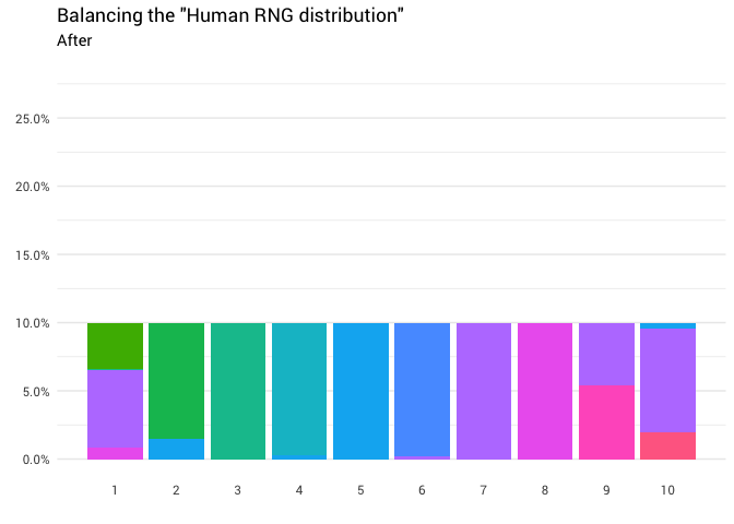
Then we transfer the problem to the solver, for example, the lpSolve package in R, combining the created constraints into a single matrix:

 # Make results reproducible... set.seed(23756434) solved <- lpSolve::lp( direction = "max", objective.in = objective, const.mat = do.call(rbind, c(constrain_original_conserved, constrain_uniform_output)), const.dir = c(rep_len("==", length(constrain_original_conserved)), rep_len("==", length(constrain_uniform_output))), const.rhs = c(rep_len(1, length(constrain_original_conserved)), rep_len(1 / nrow(probabilities), length(constrain_uniform_output))) ) balanced_probabilities <- variables %>% mutate(p = solved$solution) %>% left_join(probabilities, by = c("from" = "outcome"), suffix = c("_redistributed", "_original")) 

The following redistribution is returned:

 library(gganimate) redistribute_anim <- bind_rows(balanced_probabilities %>% mutate(key = from, state = "Before"), balanced_probabilities %>% mutate(key = to, state = "After")) %>% ggplot(aes(x = key, y = p_redistributed * p_original)) + geom_col(aes(fill = as.factor(from)), position = position_stack()) + scale_x_continuous(breaks = 1:10) + scale_y_continuous(labels = scales::percent_format(), breaks = seq(0, 1, 0.05)) + scale_fill_discrete(h = c(120, 360)) + theme_minimal(base_family = "Roboto") + theme(legend.position = "none", panel.grid.major.x = element_blank(), panel.grid.minor.x = element_blank()) + labs(title = 'Balancing the "Human RNG distribution"', subtitle = "{closest_state}", x = "", y = NULL) + transition_states( state, transition_length = 4, state_length = 3 ) + ease_aes('cubic-in-out') animate( redistribute_anim, start_pause = 8, end_pause = 8 ) 

Fine! Now we have a redistribution function. Let's take a closer look at exactly how mass moves:

 balanced_probabilities %>% ggplot(aes(x = from, y = to)) + geom_tile(aes(alpha = p_redistributed, fill = as.factor(from))) + geom_text(aes(label = ifelse(p_redistributed == 0, "", scales::percent(p_redistributed, 2)))) + scale_alpha_continuous(limits = c(0, 1), range = c(0, 1)) + scale_fill_discrete(h = c(120, 360)) + scale_x_continuous(breaks = 1:10) + scale_y_continuous(breaks = 1:10) + theme_minimal(base_family = "Roboto") + theme(panel.grid.minor = element_blank(), panel.grid.major = element_line(linetype = "dotted"), legend.position = "none") + labs(title = "Probability mass redistribution", x = "Original number", y = "Redistributed number") 

This diagram says that in about 8% of cases, when someone calls eight as a random number, you need to take the answer as a unit. In the remaining 92% of cases, it remains the number eight.

It would be quite simple to solve the problem if we had access to a generator of uniformly distributed random numbers (from 0 to 1). But we only have a room full of people. Fortunately, if you are ready to come to terms with a few minor inaccuracies, then you can make a pretty good RNG out of people without asking more than two times.

Returning to our original distribution, we have the following probabilities for each number that can be used to reassign any probabilities, if necessary.

 probabilities %>% transmute(number = outcome, probability = scales::percent(p)) 

  ## # A tibble: 10 x 2
 ## number probability
 ## <dbl> <chr>
 ## 1 1 3.4%
 ## 2 2 8.5%
 ## 3 3 10.0%
 ## 4 4 9.7%
 ## 5 5 12.2%
 ## 6 6 9.8%
 ## 7 7 28.1%
 ## 8 8 10.9%
 ## 9 9 5.4%
 ## 10 10 1.9% 

For example, when someone gives us eight as a random number, you need to determine whether this eight should be one or not (probability 8%). If we ask another person about a random number, then with a probability of 8.5% he will answer “two”. So if this second number is 2, we know that we must return 1 as a uniformly distributed random number.

Spreading this logic on all numbers, we get the following algorithm:

• Ask a person a random number $$$n_1$.
• $$$n_1 = 1, 2, 3, 4, 6, 9,$or $$$10$:
  
  • Your random number $$$n_1$
• If a $$$n_1 = 5$:
  
  • Ask another person a random number ( $$$n_2$)
  • If a $$$n_2 = 5$(12.2%):
    
    • Your random number is 2
  • If a $$$n_2 = 10$(1.9%):
    
    • Your random number is 4
  • Otherwise, your random number is 5
• If a $$$n_1 = 7$:
  
  • Ask another person a random number ( $$$n_2$)
  • If a $$$n_2 = 2$or $$$5$(20.7%):
    
    • Your random number 1
  • If a $$$n_2 = 8$or $$$9$(16.2%):
    
    • Your random number is 9
  • If a $$$n_2 = 7$(28.1%):
    
    • Your random number is 10
  • Otherwise, your random number is 7
• If a $$$n_1 = 8$:
  
  • Ask another person a random number ( $$$n_2$)
  • If a $$$n_2 = 2$(8.5%):
    
    • Your random number 1
  • Otherwise, your random number is 8

According to this algorithm, you can use a group of people to get something close to a generator of uniformly distributed random numbers from 1 to 10!