SQL: working time problem solving

Hello, Radio SQL is on the air again! Today we have a solution to the problem that we transmitted in our previous broadcast, and promised to make out the next time. And this next time has come.

The task provoked a lively response from the humanoids of the Milky Way galaxy (and not surprisingly, with their labor slavery, which they still honor for the benefit of civilization). Unfortunately, on the third planet they delayed the launch of the Space Observatory "Spectr-RG" at the end of July 2019 PX (local chronology), with the help of which it was planned to broadcast this program. I had to look for alternative transmission routes, which led to a slight delay in the signal. But all is well that ends well.

At once I will say that there will be no magic in the analysis of the task, there is no need to look for revelations here or to wait for some particularly effective (or some other in any other sense) implementation. This is just a parsing task. In it, those who do not know how to approach the solution of such problems will be able to see how to solve them. Moreover, there is nothing terrible here.

with periods(id, start_time, stop_time) as ( values(1, '2019-03-29 07:00:00'::timestamp, '2019-04-08 14:00:00'::timestamp), (2, '2019-04-10 07:00:00'::timestamp, '2019-04-10 20:00:00'::timestamp), (3, '2019-04-11 12:00:00'::timestamp, '2019-04-12 16:07:12'::timestamp), (4, '2018-12-28 12:00:00'::timestamp, '2019-01-16 16:00:00'::timestamp) ) 

  id | start_time | stop_time | work_hrs ----+---------------------+---------------------+---------- 1 | 2019-03-29 07:00:00 | 2019-04-08 14:00:00 | 58:00:00 2 | 2019-04-10 07:00:00 | 2019-04-10 20:00:00 | 09:00:00 3 | 2019-04-11 12:00:00 | 2019-04-12 16:07:12 | 13:07:12 4 | 2018-12-28 12:00:00 | 2019-01-16 16:00:00 | 67:00:00 

The light piquancy of the task is given by the fact that I quite consciously gave a good half of the condition in a descriptive form (as is usually the case in real life), leaving the technical implementation to the discretion of the decider, how exactly the work schedule should be set. On the one hand, this requires some architectural thinking skills. On the other hand, the ready-made format of this schedule would already have prompted some of its template use. And if you omit, the thought and imagination will work more fully. The reception paid off completely, allowing me, too, to find interesting approaches in published solutions.

So, to solve the original problem in this way, two subtasks will need to be solved:

1. Determine how to define the work schedule most compactly, moreover so that it is convenient to use them for the solution.
2. Actually calculate the duration of each initial period in working hours on a working schedule from the previous subtask.

And it is better to start with the second, in order to understand in what form we need to solve the first. Then decide the first and return again to the second, to get the final result.
We will gradually collect the result, using the CTE syntax, which allows you to put all the necessary data samples into separate named subqueries, and then put everything together.

Well, let's go.

Calculate the duration in working hours

To calculate the duration of each of the periods in working hours in the forehead, you need to cross the initial period (green color on the diagram) with intervals that describe the working time (orange). Working time intervals are Mondays from 10:00 to 19:00, Tuesdays from 10:00 to 19:00, and so on. The result is shown in blue:

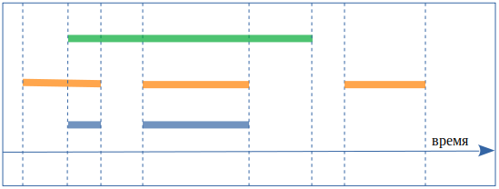
By the way, in order to be less confused, I will always refer to the original periods as periods, and I will call the working time intervals.

The procedure should be repeated for each initial period. We have already set the initial periods in the periods (start_time, stop_time) table , the working time will be presented as a table, say, schedule (strat_time, stop_time) , where every working day is present. The result is a complete Cartesian product of all initial periods and working time intervals.

Intersections can be calculated in the classical way, having considered all possible variants of interval intersections - we cross green with orange, the result is blue:

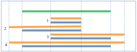
and taking each case the desired value for the beginning and end of the result:

  select s.start_time, s.stop_time -- case #1 from periods p, schedule s where p.start_time <= s.start_time and p.stop_time > s.stop_time union all select p.start_time, s.stop_time -- case #2 from periods p, schedule s where p.start_time >= s.start_time and p.stop_time > s.stop_time and p.start_time < s.stop_time union all select s.start_time, p.stop_time -- case #3 from periods p, schedule s where p.start_time <= s.start_time and p.stop_time < s.stop_time and p.stop_time > s.start_time union all select p.start_time, p.stop_time -- case #4 from periods p, schedule s where p.start_time >= s.start_time and p.stop_time < s.stop_time 

Since for each intersection we can only have one of the four options, they are all connected in one query with the help of union all .

You can do otherwise, using the type of tsrange available in PostgreSQL and the intersection operation already available for it:

  select tsrange(s.start_time, s.stop_time) * tsrange(s.start_time, s.stop_time) from periods p, schedule s 

Agree that so - eeee - a little easier. In general, PostgreSQL has quite a few such convenient little things, so it’s nice to write queries on it.

Generate calendar

Now let's go back to the subtask with the task schedule.

Work schedule we need to get in the form of working time intervals from 10:00 to 19:00 for each working day, something like schedule (start_time, stop_time) . As we understood, it will be convenient to solve our problem. In real life, such a schedule should be given in tabular form; for two years it’s only about 500 records; for practical purposes, even a dozen years will need to be asked - a couple with half a thousand records, is nonsense for modern databases. But we have a task that will be solved in one query, and it’s not very practical to list the entire table as a whole. Let's try to implement it more compactly.

In any case, we will need holidays in order to remove them from the basic schedule, and here only the listing is appropriate:

  dates_exclude(d) as ( values('2018-01-01'::date), -- 2018 ('2018-01-02'::date), ('2018-01-03'::date), ('2018-01-04'::date), ('2018-01-05'::date), ('2018-01-08'::date), ('2018-02-23'::date), ('2018-03-08'::date), ('2018-03-09'::date), ('2018-05-01'::date), ('2018-05-02'::date), ('2018-05-09'::date), ('2018-06-11'::date), ('2018-06-12'::date), ('2018-11-05'::date), ('2018-12-31'::date), ('2019-01-01'::date), -- 2019 ('2019-01-02'::date), ('2019-01-03'::date), ('2019-01-04'::date), ('2019-01-07'::date), ('2019-01-08'::date), ('2019-03-08'::date), ('2019-05-01'::date), ('2019-05-02'::date), ('2019-05-03'::date), ('2019-05-09'::date), ('2019-05-10'::date), ('2019-06-12'::date), ('2019-11-04'::date) ) 

and additional business days to add:

  dates_include(d) as ( values --  2018,  2019  ('2018-04-28'::date), ('2018-06-09'::date), ('2018-12-29'::date) ) 

The sequence of working days for two years can be generated by a special and very suitable function generate_series () , immediately incidentally throwing out Saturdays and Sundays:

  select d from generate_series( '2018-01-01'::timestamp , '2020-01-01'::timestamp , '1 day'::interval ) as d where extract(dow from d) not in (0,6) --     

We will get working days by connecting everything together: we generate a sequence of all working days in two years, add additional working days from dates_include and remove all additional days from dates_exclude :

  schedule_base as ( select d from generate_series( '2018-01-01'::timestamp , '2020-01-01'::timestamp , '1 day'::interval ) as d where extract(dow from d) not in (0,6) --     union select d from dates_include --     except select d from dates_exclude --     ) 

And now we get the working time intervals we need:

  schedule(start_time, stop_time) as ( select d + '10:00:00'::time, d + '19:00:00'::time from schedule_base ) 

So, the schedule received.

Putting it all together

Now we will get the intersection:

  select p.* , tsrange(p.start_time, p.stop_time) * tsrange(s.start_time, s.stop_time) as wrkh from periods p join schedule s on tsrange(p.start_time, p.stop_time) && tsrange(s.start_time, s.stop_time) 

Pay attention to the join condition ON , it does not match two corresponding records from the joined tables, such a match does not exist, but some optimization is introduced that cuts off the working time intervals with which our initial period does not overlap. This is done using the && operator, which checks the intersection of tsrange intervals. This removes a mass of empty intersections so that they do not interfere in front of the eyes, but, on the other hand, removes information about those initial periods that fall entirely on nonworking time. So we admire our approach and rewrite the query like this:

  periods_wrk as ( select p.* , tsrange(p.start_time, p.stop_time) * tsrange(s.start_time, s.stop_time) as wrkh from periods p , schedule s ) select id, start_time, stop_time , sum(upper(wrkh)-lower(wrkh)) from periods_wrk group by id, start_time, stop_time 

In periods_wrk we decompose each initial period into working intervals, and then we count their total duration. It turned out a complete Cartesian product of all periods at intervals, but no period was lost.

Everything, the result is received. NULL values ​​for empty intervals were not pleasant; let the query show a zero-length interval better. Check the amount in coalesce () :

 select id, start_time, stop_time , coalesce(sum(upper(wrkh)-lower(wrkh)), '0 sec'::interval) from periods_wrk group by id, start_time, stop_time 

All together gives the final result:

 with periods(id, start_time, stop_time) as ( values(1, '2019-03-29 07:00:00'::timestamp, '2019-04-08 14:00:00'::timestamp) , (2, '2019-04-10 07:00:00'::timestamp, '2019-04-10 20:00:00'::timestamp) , (3, '2019-04-11 12:00:00'::timestamp, '2019-04-12 16:00:00'::timestamp) , (4, '2018-12-28 12:00:00'::timestamp, '2019-01-16 16:00:00'::timestamp) ), dates_exclude(d) as ( values('2018-01-01'::date), -- 2018 ('2018-01-02'::date), ('2018-01-03'::date), ('2018-01-04'::date), ('2018-01-05'::date), ('2018-01-08'::date), ('2018-02-23'::date), ('2018-03-08'::date), ('2018-03-09'::date), ('2018-05-01'::date), ('2018-05-02'::date), ('2018-05-09'::date), ('2018-06-11'::date), ('2018-06-12'::date), ('2018-11-05'::date), ('2018-12-31'::date), ('2019-01-01'::date), -- 2019 ('2019-01-02'::date), ('2019-01-03'::date), ('2019-01-04'::date), ('2019-01-07'::date), ('2019-01-08'::date), ('2019-03-08'::date), ('2019-05-01'::date), ('2019-05-02'::date), ('2019-05-03'::date), ('2019-05-09'::date), ('2019-05-10'::date), ('2019-06-12'::date), ('2019-11-04'::date) ), dates_include(start_time, stop_time) as ( values --  2018,  2019  ('2018-04-28 10:00:00'::timestamp, '2018-04-28 19:00:00'::timestamp), ('2018-06-09 10:00:00'::timestamp, '2018-06-09 19:00:00'::timestamp), ('2018-12-29 10:00:00'::timestamp, '2018-12-29 19:00:00'::timestamp) ) ), schedule_base(start_time, stop_time) as ( select d::timestamp + '10:00:00', d::timestamp + '19:00:00' from generate_series( (select min(start_time) from periods)::date::timestamp , (select max(stop_time) from periods)::date::timestamp , '1 day'::interval ) as days(d) where extract(dow from d) not in (0,6) ), schedule as ( select * from schedule_base where start_time::date not in (select d from dates_exclude) union select * from dates_include ), periods_wrk as ( select p.* , tsrange(p.start_time, p.stop_time) * tsrange(s.start_time, s.stop_time) as wrkh from periods p , schedule s ) select id, start_time, stop_time , sum(coalesce(upper(wrkh)-lower(wrkh), '0 sec'::interval)) from periods_wrk group by id, start_time, stop_time 

Hooray! .. This could be finished, but for completeness we will consider some more related topics.

Further development of the topic

Shortened pre-holiday days, lunch breaks, different schedules for different days of the week ... In principle, everything is clear, you need to correct the definition of the schedule , just give a couple of examples.

This is how you can set different times for the beginning and end of the working day depending on the day of the week:

  select d + case extract(dow from d) when 1 then '10:00:00'::time --  when 2 then '11:00:00'::time --  when 3 then '11:00:00'::time --  --        else '10:00:00'::time end , d + case extract(dow from d) --   19   when 5 then '14:00:00'::time --  else '19:00:00'::time end from schedule_base 

If you need to take into account lunch breaks from 13:00 to 14:00, then instead of one interval per day, we do two:

  select d + '10:00:00'::time , d + '13:00:00'::time from schedule_base union all select d + '14:00:00'::time , d + '19:00:00'::time from schedule_base 

Well, and so on.

Performance

I will say a few words about performance, as there are always questions about it. I will not chew much here, this is a section with an asterisk.

In general, premature optimization is evil. According to my many years of observations, the readability of a code is its main advantage. If the code is well read, then it is easier to maintain and develop. Well readable code implicitly requires both a good solution architecture, and proper commenting, and successful variable names, compactness not at the expense of readability, etc., that is, everything for which the code is called good.

Therefore, we always write the query as readable as possible, and we start optimizing if and only if it turns out that the performance is insufficient. And we will optimize exactly where the performance will be insufficient and exactly to the extent that it becomes sufficient. If you certainly value your own time, and you have something to do.

But not to do extra work in the request - this is correct, you should always try to take this into account.

Based on this, we will include one optimization in the query right away - let each initial period intersect only with those working time intervals with which it has common points (instead of the long classical condition on the boundaries of the range, it is more convenient to use the built-in && operator for tsrange type). This optimization has already appeared in the request, but has led to the fact that the initial periods have disappeared from the results, which completely fell on the non-working time.

We will return this optimization back. To do this, use the LEFT JOIN , which saves all the records from the periods table. Now the periods_wrk subquery will look like this:

 , periods_wrk as ( select p.* , tsrange(p.start_time, p.stop_time) * tsrange(s.start_time, s.stop_time) as wrkh from periods p left join schedule s on tsrange(p.start_time, p.stop_time) && tsrange(s.start_time, s.stop_time)) 

Analysis of the query shows that the time on the test data has decreased approximately by half. Since the execution time depends on what the server was doing at the same time, I took a few measurements and gave some “typical” result, not the biggest, not the smallest, from the middle.

Old query:

 explain (analyse) with periods(id, start_time, stop_time) as ( ... QUERY PLAN ------------------------------------------------------------------------------------ HashAggregate (cost=334.42..338.39 rows=397 width=36) (actual time=10.724..10.731 rows=4 loops=1) ... 

New:

 explain (analyse) with periods(id, start_time, stop_time) as ( ... QUERY PLAN ------------------------------------------------------------------------------------ HashAggregate (cost=186.37..186.57 rows=20 width=36) (actual time=5.431..5.440 rows=4 loops=1) ... 

But the most important thing is that such a query will also be scaled better, requiring less server resources, since the full Cartesian product grows very quickly.

And on this I would stop with optimizations. When I solved this task for myself, I had enough performance even in much more terrible form of this query, but there really was no need to optimize. To get a report on my data once a quarter, I can wait an extra ten seconds. Spent on optimization an extra hour of time in such conditions will never pay off.

But it turns out to be uninteresting, let's still think about how events could develop if the optimization in terms of execution time would really be needed. For example, we want to monitor this parameter in real time for each of our records in the database, that is, for every such request will be called. Well, or think of your reason, why would need to optimize.

The first thing that comes to mind is to count once and put a table with working intervals into the database. There may be contraindications: if the base can not be changed, or difficulties are expected with the support of current data in such a table. Then it will have to leave the generation of working time "on the fly" in the request itself, the benefit is not too heavy subquery.

The next and most powerful (but not always applicable) approach is algorithmic optimization. Some of these approaches have already been presented in the comments to the article with the condition of the problem.

I like this one more than anything else. If you make a table with all (not only working) days of the calendar and calculate as a cumulative total, how many working hours have passed from a certain “creation of the world”, then you can get the number of working hours between two dates by one subtraction operation. It only remains to correctly take into account the working time for the first and last day - and it is ready. Here's what I got in this approach:

  schedule_base(d, is_working) as ( select '2018-01-01'::date, 0 union all select d+1, case when extract(dow from d+1) not in (0,6) and d+1 <> all('{2019-01-01,2019-01-02,2019-01-03,2019-01-04,2019-01-07,2019-01-08,2019-03-08,2019-05-01,2019-05-02,2019-05-03,2019-05-09,2019-05-10,2019-06-12,2019-11-04,2018-01-01,2018-01-02,2018-01-03,2018-01-04,2018-01-05,2018-01-08,2018-02-23,2018-03-08,2018-03-09,2018-04-30,2018-05-01,2018-05-02,2018-05-09,2018-06-11,2018-06-12,2018-11-05,2018-12-31}') or d+1 = any('{2018-04-28,2018-06-09,2018-12-29}') then 1 else 0 end from schedule_base where d < '2020-01-01' ), schedule(d, is_working, work_hours) as ( select d, is_working , sum(is_working*'9 hours'::interval) over (order by d range between unbounded preceding and current row) from schedule_base ) select p.* , s2.work_hours - s1.work_hours + ('19:00:00'::time - least(greatest(p.start_time::time, '10:00:00'::time), '19:00:00'::time)) * s1.is_working - ('19:00:00'::time - least(greatest(p.stop_time::time, '10:00:00'::time), '19:00:00'::time)) * s2.is_working as wrk from periods p, schedule s1, schedule s2 where s1.d = p.start_time::date and s2.d = p.stop_time::date 

Let me briefly explain what is happening here. In the schedule_base subquery, we generate all calendar days in two years, and by each day we determine the sign of whether the working day is (= 1) or not (= 0). Further in the schedule subquery, we consider the window function the cumulative total number of working hours from 2018-01-01. It would be possible to do everything in one subquery, but it would be more cumbersome, which would worsen readability. Then in the main query we consider the difference between the number of working hours at the end and the beginning of the period and, somewhat floridly, we consider the working time for the first and last day of the period. The intricacy is related to the time shift before the beginning of the working day to its beginning, and the time after the end of the working day to its end. And if part of the query with shedule_base and schedule is removed to a separate, pre-calculated table of the hotel (as suggested earlier), the query will turn into a completely trivial one.

Let's compare the execution on the larger sample in order to better demonstrate the optimization done, on four periods the task condition takes more time to generate a work schedule.

I took about 3 thousand periods. I will give only the top total line in EXPLAIN, typical values ​​are as follows.

Original version:

 GroupAggregate (cost=265790.95..296098.23 rows=144320 width=36) (actual time=656.654..894.383 rows=2898 loops=1) ... 

Optimized:

 Hash Join (cost=45.01..127.52 rows=70 width=36) (actual time=1.620..5.385 rows=2898 loops=1) ... 

The gain in time turned out a couple of orders of magnitude. With the increase in the number of periods and their length in years, the gap will only increase.

It would seem all is well, but why, having made such optimization, I left the first variant of the query for myself until its performance was enough? Because the optimized version is undoubtedly faster, but it takes much more time to understand how it works, that is, readability has deteriorated. That is, the next time when I need to rewrite the query under my changed conditions, I (or not) will have to spend significantly more time on understanding how the query works.

At this all today, keep the tentacles warm, and I say goodbye to you until the next release of SQL Radio.