Sampling and calculation accuracy
A number of my colleagues are faced with the problem that in order to calculate a certain metric, for example, a conversion rate, it is necessary to check the entire database. Or you need to conduct detailed research on each client, where there are millions of customers. These kinds of checks can work for quite a long time, even in storage facilities specially made for this. It's not very cool to wait for 5-15-40 minutes, while a simple metric is considered to find out that you need to count something else or add something else.
Sampling is one of the solutions to this problem: we are not trying to calculate our metric on the whole data array, but take a subset that representatively represents the metrics we need. This sample can be 1000 times smaller than our data set, but at the same time it is good enough to show the numbers we need.
In this article, I decided to demonstrate how the sampling sample sizes affect the final metric error.
Problem
The key question is: how well does the sample describe the “population”? Once we take a sample from the common array, the metrics we get are random variables. Different samples will give us different metrics results. Different, does not mean any. Probability theory tells us that sampling metric values should be grouped around the true metric value (taken over the entire sample) with a certain level of error. At the same time, we often have problems where, to solve, we can manage with different levels of error. It's one thing to figure out whether we get a conversion of 50% or 10%, and another thing is to get the result with an accuracy of 50.01% vs 50.02%.
Interestingly, from the point of view of the theory, the conversion rate observed by us over the entire sample is also a random variable, since The “theoretical” conversion rate can only be calculated on a sample of infinite size. This means that even all our observations in the database actually give an estimate of the conversion with their accuracy, although it seems to us that these calculated figures of ours are absolutely accurate. This also leads to the conclusion that even if today the conversion rate is different from yesterday's, it does not mean that something has changed, but only means that today's sample (all observations in the database) from the general population (all possible observations of this day, which occurred and did not occur) gave a slightly different result than yesterday. In any case, for any honest product or analyst, this should be a basic hypothesis.
Task statement
Suppose we have 1,000,000 entries in the database of the form 0/1, which tell us about whether there was a conversion on the event. Then the conversion rate is simply the sum of 1 divided by 1 million.
Question: if we take a sample of size N, then by how much and with what probability will the conversion rate differ from that calculated for the entire sample?
Theoretical reasoning
The task is to calculate the confidence interval of the conversion coefficient for a sample of a given size for the binomial distribution.
From theory, the standard deviation for the binomial distribution is:
S = sqrt (p * (1 - p) / N)
Where
p - conversion rate
N - sample size
S - standard deviation
I will not take the confidence interval directly from the theory. There is a rather complicated and tangled mat, which ultimately relates the standard deviation and the final estimate of the confidence interval.
Let's develop an "intuition" about the standard deviation formula:
- The larger the sample size, the smaller the error. In this case, the error falls in the inverse quadratic dependence, i.e. an increase in the sample by 4 times increases the accuracy only 2 times. This means that at some point, increasing the sample size will not give special advantages, and also means that a fairly high accuracy can be obtained with a rather small sample.

- There is an error dependence on the conversion rate. The relative error (i.e., the ratio of the error to the magnitude of the conversion rate) has the “nasty” tendency to be the greater, the lower the conversion rate:
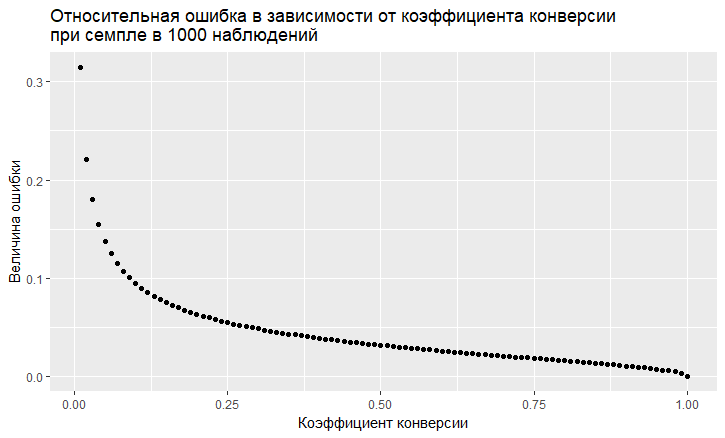
- As we can see, the error "flies up" into the sky with a low conversion rate. This means that if you sample rare events, then you need large sample sizes, otherwise you will get a conversion estimate with a very large error.
Modeling
We can completely move away from the theoretical solution and solve the problem "head on." Thanks to the R language, this is now very easy to do. To answer the question of which error we get in sampling, you can simply do a thousand samples and see what error we get.
The approach is as follows:
- We take different conversion rates (from 0.01% to 50%).
- We take 1000 samples of 10, 100, 1000, 10000, 50000, 100000, 250000, 500000 elements in the sample
- We count the conversion rate for each group of samples (1000 coefficients)
- We build a histogram for each group of samples and determine the extent to which 60%, 80% and 90% of the observed conversion rates lie.
Code on R that generates data:
sample.size <- c(10, 100, 1000, 10000, 50000, 100000, 250000, 500000) bootstrap = 1000 Error <- NULL len = 1000000 for (prob in c(0.0001, 0.001, 0.01, 0.1, 0.5)){ CRsub <- data.table(sample_size = 0, CR = 0) v1 = seq(1,len) v2 = rbinom(len, 1, prob) set = data.table(index = v1, conv = v2) print(paste('probability is: ', prob)) for (j in 1:length(sample.size)){ for(i in 1:bootstrap){ ss <- sample.size[j] subset <- set[round(runif(ss, min = 1, max = len),0),] CRsample <- sum(subset$conv)/dim(subset)[1] CRsub <- rbind(CRsub, data.table(sample_size = ss, CR = CRsample)) } print(paste('sample size is:', sample.size[j])) q <- quantile(CRsub[sample_size == ss, CR], probs = c(0.05,0.1, 0.2, 0.8, 0.9, 0.95)) Error <- rbind(Error, cbind(prob,ss,t(q))) } As a result, we get the following table (more will be the graphics, but the details are better seen in the table).
| Conversion rate | Sample size | five% | ten% | 20% | 80% | 90% | 95% |
|---|---|---|---|---|---|---|---|
| 0.0001 | ten | 0 | 0 | 0 | 0 | 0 | 0 |
| 0.0001 | 100 | 0 | 0 | 0 | 0 | 0 | 0 |
| 0.0001 | 1000 | 0 | 0 | 0 | 0 | 0 | 0.001 |
| 0.0001 | 10,000 | 0 | 0 | 0 | 0.0002 | 0.0002 | 0.0003 |
| 0.0001 | 50,000 | 0.00004 | 0.00004 | 0.00006 | 0.00014 | 0.00016 | 0.00018 |
| 0.0001 | 100,000 | 0.00005 | 0.00006 | 0.00007 | 0.00013 | 0.00014 | 0.00016 |
| 0.0001 | 250,000 | 0.000072 | 0.0000796 | 0.000088 | 0.00012 | 0.000128 | 0.000136 |
| 0.0001 | 500,000 | 0.00008 | 0.000084 | 0.000092 | 0.000114 | 0.000122 | 0.000128 |
| 0.001 | ten | 0 | 0 | 0 | 0 | 0 | 0 |
| 0.001 | 100 | 0 | 0 | 0 | 0 | 0 | 0.01 |
| 0.001 | 1000 | 0 | 0 | 0 | 0.002 | 0.002 | 0.003 |
| 0.001 | 10,000 | 0.0005 | 0.0006 | 0.0007 | 0.0013 | 0.0014 | 0.0016 |
| 0.001 | 50,000 | 0.0008 | 0.000858 | 0.00092 | 0.00116 | 0.00122 | 0.00126 |
| 0.001 | 100,000 | 0.00087 | 0.00091 | 0.00095 | 0.00112 | 0.00116 | 0.0012105 |
| 0.001 | 250,000 | 0.00092 | 0.000948 | 0.000972 | 0.001084 | 0.001116 | 0.0011362 |
| 0.001 | 500,000 | 0.000952 | 0.0009698 | 0.000988 | 0.001066 | 0.001086 | 0.0011041 |
| 0.01 | ten | 0 | 0 | 0 | 0 | 0 | 0.1 |
| 0.01 | 100 | 0 | 0 | 0 | 0.02 | 0.02 | 0.03 |
| 0.01 | 1000 | 0.006 | 0.006 | 0.008 | 0.013 | 0.014 | 0.015 |
| 0.01 | 10,000 | 0.0086 | 0.0089 | 0.0092 | 0.0109 | 0.0114 | 0.0118 |
| 0.01 | 50,000 | 0.0093 | 0.0095 | 0.0097 | 0.0104 | 0.0106 | 0.0108 |
| 0.01 | 100,000 | 0.0095 | 0.0096 | 0.0098 | 0.0103 | 0.0104 | 0.0106 |
| 0.01 | 250,000 | 0.0097 | 0.0098 | 0.0099 | 0.0102 | 0.0103 | 0.0104 |
| 0.01 | 500,000 | 0.0098 | 0.0099 | 0.0099 | 0.0102 | 0.0102 | 0.0103 |
| 0.1 | ten | 0 | 0 | 0 | 0.2 | 0.2 | 0.3 |
| 0.1 | 100 | 0.05 | 0.06 | 0.07 | 0.13 | 0.14 | 0.15 |
| 0.1 | 1000 | 0.086 | 0.0889 | 0.093 | 0.108 | 0.1121 | 0.117 |
| 0.1 | 10,000 | 0.0954 | 0.0963 | 0.0979 | 0.1028 | 0.1041 | 0.1055 |
| 0.1 | 50,000 | 0.098 | 0.0986 | 0.0992 | 0.1014 | 0.1019 | 0.1024 |
| 0.1 | 100,000 | 0.0987 | 0.099 | 0.0994 | 0.1011 | 0.1014 | 0.1018 |
| 0.1 | 250,000 | 0.0993 | 0.0995 | 0.0998 | 0.1008 | 0.1011 | 0.1013 |
| 0.1 | 500,000 | 0.0996 | 0.0998 | 0.1 | 0.1007 | 0.1009 | 0.101 |
| 0.5 | ten | 0.2 | 0.3 | 0.4 | 0.6 | 0.7 | 0.8 |
| 0.5 | 100 | 0.42 | 0.44 | 0.46 | 0.54 | 0.56 | 0.58 |
| 0.5 | 1000 | 0.473 | 0.478 | 0.486 | 0.513 | 0.52 | 0.525 |
| 0.5 | 10,000 | 0.4922 | 0.4939 | 0.4959 | 0.5044 | 0.5061 | 0.5078 |
| 0.5 | 50,000 | 0.4962 | 0.4968 | 0.4978 | 0.5018 | 0.5028 | 0.5036 |
| 0.5 | 100,000 | 0.4974 | 0.4979 | 0.4986 | 0.5014 | 0.5021 | 0.5027 |
| 0.5 | 250,000 | 0.4984 | 0.4987 | 0.4992 | 0.5008 | 0.5013 | 0.5017 |
| 0.5 | 500,000 | 0.4988 | 0.4991 | 0.4994 | 0.5006 | 0.5009 | 0.5011 |
Consider cases with 10% conversion and low 0.01% conversion, since they are clearly visible all the features of working with sampling.
At 10% conversion, the picture looks pretty simple:

The points are the edges of the 5-95% confidence interval, i.e. making a sample in 90% of cases we will receive CR on a sample within this interval. The vertical scale is the sample size (logarithmic scale), the horizontal one is the value of the conversion rate. The vertical bar is the "true" CR.
Here we see the same thing that we saw from the theoretical model: accuracy increases as the sample size grows, while one fairly "converges" and the sample gets a result close to the "true" one. A total of 1000 samples, we have 8.6% - 11.7%, which for a number of tasks will be enough. And on 10 thousand already 9.5% - 10.55%.
Things are worse with rare events and this is consistent with the theory:

A low conversion rate of 0.01% has a problem with statistics of 1 million observations, and with samples the situation is even worse. The error becomes simply gigantic. In samples up to 10,000, the metric is not valid in principle. For example, in a sample of 10 observations, my generator simply received 0 times a 1000 conversion, so there is only 1 point. On 100 thousand we have a range from 0.005% to 0.0016%, that is, we can make a mistake by almost half the coefficient with this sampling.
It is also worth noting that when you see conversion of such a small scale per 1 million tests, then you have just a big natural error. From this it follows that conclusions on the dynamics of such rare events should be made on really large samples, otherwise you just chase ghosts, random fluctuations in the data.
Findings:
- Sampling working method to get estimates
- The accuracy of the samples increases with increasing sample size and decreases with a decrease in the conversion rate.
- The accuracy of the estimates can be modeled for your task and thus choose the best sampling for yourself.
- It is important to remember that rare events sample badly.
- In general, rare events are difficult to analyze, they require large data samples without samples.
')
Source: https://habr.com/ru/post/458890/
All Articles