Noise in big data. Entropy-based analysis
There was a task called “ Enskomba Quartet ( Anskomba )” ( English version ).
Figure 1 shows the tabular distribution of 4 random functions (taken from Wikipedia).

Fig. 1. Tabular distribution of four random functions
')
Figure 2 shows the distribution parameters of these random functions.

Fig. 2. Parameters of distributions of four random functions
And their graphs in Figure 3.
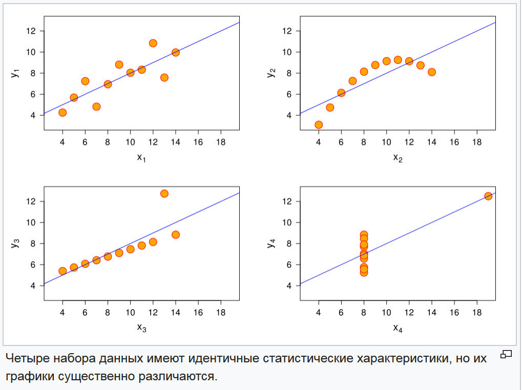
Fig. 3. Plots of four random functions
The problem of distinguishing these functions is solved quite simply by comparing higher- order moments and their normalized indices: the asymmetry coefficient and the kurtosis coefficient. These indicators are presented in Figure 4.

Fig. 4. Indicators of the moments of the third and fourth order and the coefficients of asymmetry and kurtosis of four random functions
As can be seen from the table in Figure 4, the combination of these indicators is different for all functions.
The first conclusion, which naturally suggested itself, is that the information on the relative position of the points is stored in the distribution parameters at a higher level than the variance of the random distribution.
Many analysts are trying to isolate particular regression equations in big data and so far, to date, this is by selecting the equation with the least residual variance. There is not much to add. But he paid attention to the fact that this is all information, and information has an indicator of entropy . And it, entropy, has its limits from 0, when the information is completely defined to white noise. And white noise, in the transmission channel, has a uniform distribution.
When data is required to be analyzed, it is initially assumed that they contain related data that need to be formalized as a relationship. This suggests that the data are not white noise. That is, the first stage is the selection of the regression equation and the determination of the residual variance. If the regression is chosen correctly, then the residual variance will obey the law of normal distribution. Let us see and, in Figures 5-7, the entropy formulas for a uniformly distributed and normally distributed random variable are presented.

Fig. 5. The formula of differential entropy for a normally distributed quantity (Afanasyev V.V. Theory of Probability in Questions and Tasks . The Ministry of Education and Science of the Russian Federation Yaroslavl State Pedagogical University named after KD Ushinsky)

Fig. 6. The formula for differential entropy for a normally distributed quantity (Pugachev VS Theory of random functions and its application to automatic control problems . Ed. 2nd, revised and enlarged. - M .: Fizmatlit, 1960. - 883 p.)

Fig. 7. The formula of differential entropy for a uniformly distributed quantity (Pugachev VS The theory of random functions and its application to the problems of automatic control . Ed. 2nd, revised and additional. - M .: Fizmatlit, 1960. - 883 p.)
Next, we show an example. But first we take the conditions that each of the four functions is the coordinate of the hyperplane, that is, at the same time we will check the work of the model in multidimensional space. Perform a convolution of the hypercube to the plane. The mechanism is presented in Figure 8.


Fig. 8. Baseline data with convolution mechanism

Fig. 9. Summary group in the figure.

Fig. 10. Parameters of distributions of four random functions and consolidated grouping.
Consider the mechanism for choosing the value of the partition interval. The initial conditions are shown in Figure 11.

Fig. 11. The initial conditions of splitting into intervals.
Condition 1. It must be with a non-zero probability on the region of variation, since otherwise, the entropy is infinity. Both for the initial sample and for the residual one.
Condition 2. Since it is impossible to ignore the possibility of an outlier, in the new data, etc., then for the extreme intervals, it is necessary to establish the probability according to the normal or other generally accepted theoretical law of probability distribution, according to the principle of the probability of tails.
Condition 3. The interval step should provide the minimum number of intervals required for the residual sample spread.
Condition 4. The number of intervals must be odd.
Condition 5. The number of intervals must ensure reliable agreement with the theoretical distribution law chosen for the study.

Fig. 12. Residual distribution series
Define the mechanism for selecting intervals in Figure 13.

Fig. 13. Interval selection algorithm
The main problem, in my opinion, was deciding whether to enter tail intervals or not. If it looked natural enough for the residual dispersion, it was sufficiently tight for the main series.

Fig. 14. The results of processing data values in determining the information entropy
Comparing the resulting indicators of the table in Figure 14, it can be seen that they reacted to a change in the data structure. This means that the instrument has sensitivity, and allows solving problems similar to the problem of the Enskimb Quartet.
Without a doubt, these tasks can be solved with the help of higher-order moments. But in its essence, informational entropy depends on the dispersion of a random variable, that is, it is an external characteristic of dispersion. This means that we can specify the intervals where the use of analysis of variance can lead to a specific result.
The numerical characteristic of entropy makes it possible to conduct a correlation analysis with independent variables. As one example of the manifestation of a possible connection, the following: Suppose, in the interval from a to b, the noise level of the data series increased significantly, comparing the values of independent variables, found that the variable xn was in the range of more than 5 units, after it variable, decreased below +5, noise decreased. Further, we can make an additional check and, if this hypothesis is confirmed, then in further studies to prohibit the variable xn to rise above +5. Since in this case, the data becomes useless.
I assume that there are other options for using this tool.
In this aspect, the natural mechanism of the “moving average” is seen; I suppose that the sample size obtained by the formula for the sample size from statistical analysis will give a reasonable amount of the slip area. According to the current analysis, it was concluded that the sample size should be determined from the minimum fraction that falls on with the least probability. In our example, for the residual dispersion, the minimum fraction of the empirical range is 0.15909. This must be done, because if some interval in the slip volume is empty, then the noise figure will be beyond the limits or the rule will work that the logarithm 0 is equal to minus infinity. And with a correctly selected sample size, the exorbitant values of this indicator indicate a fundamental change in the structure of information.
Figure 1 shows the tabular distribution of 4 random functions (taken from Wikipedia).
Fig. 1. Tabular distribution of four random functions
')
Figure 2 shows the distribution parameters of these random functions.
Fig. 2. Parameters of distributions of four random functions
And their graphs in Figure 3.
Fig. 3. Plots of four random functions
The problem of distinguishing these functions is solved quite simply by comparing higher- order moments and their normalized indices: the asymmetry coefficient and the kurtosis coefficient. These indicators are presented in Figure 4.
Fig. 4. Indicators of the moments of the third and fourth order and the coefficients of asymmetry and kurtosis of four random functions
As can be seen from the table in Figure 4, the combination of these indicators is different for all functions.
The first conclusion, which naturally suggested itself, is that the information on the relative position of the points is stored in the distribution parameters at a higher level than the variance of the random distribution.
Many analysts are trying to isolate particular regression equations in big data and so far, to date, this is by selecting the equation with the least residual variance. There is not much to add. But he paid attention to the fact that this is all information, and information has an indicator of entropy . And it, entropy, has its limits from 0, when the information is completely defined to white noise. And white noise, in the transmission channel, has a uniform distribution.
When data is required to be analyzed, it is initially assumed that they contain related data that need to be formalized as a relationship. This suggests that the data are not white noise. That is, the first stage is the selection of the regression equation and the determination of the residual variance. If the regression is chosen correctly, then the residual variance will obey the law of normal distribution. Let us see and, in Figures 5-7, the entropy formulas for a uniformly distributed and normally distributed random variable are presented.
Fig. 5. The formula of differential entropy for a normally distributed quantity (Afanasyev V.V. Theory of Probability in Questions and Tasks . The Ministry of Education and Science of the Russian Federation Yaroslavl State Pedagogical University named after KD Ushinsky)
Fig. 6. The formula for differential entropy for a normally distributed quantity (Pugachev VS Theory of random functions and its application to automatic control problems . Ed. 2nd, revised and enlarged. - M .: Fizmatlit, 1960. - 883 p.)
Fig. 7. The formula of differential entropy for a uniformly distributed quantity (Pugachev VS The theory of random functions and its application to the problems of automatic control . Ed. 2nd, revised and additional. - M .: Fizmatlit, 1960. - 883 p.)
Next, we show an example. But first we take the conditions that each of the four functions is the coordinate of the hyperplane, that is, at the same time we will check the work of the model in multidimensional space. Perform a convolution of the hypercube to the plane. The mechanism is presented in Figure 8.
Fig. 8. Baseline data with convolution mechanism
Fig. 9. Summary group in the figure.
Fig. 10. Parameters of distributions of four random functions and consolidated grouping.
Consider the mechanism for choosing the value of the partition interval. The initial conditions are shown in Figure 11.
Fig. 11. The initial conditions of splitting into intervals.
Condition 1. It must be with a non-zero probability on the region of variation, since otherwise, the entropy is infinity. Both for the initial sample and for the residual one.
Condition 2. Since it is impossible to ignore the possibility of an outlier, in the new data, etc., then for the extreme intervals, it is necessary to establish the probability according to the normal or other generally accepted theoretical law of probability distribution, according to the principle of the probability of tails.
Condition 3. The interval step should provide the minimum number of intervals required for the residual sample spread.
Condition 4. The number of intervals must be odd.
Condition 5. The number of intervals must ensure reliable agreement with the theoretical distribution law chosen for the study.
Fig. 12. Residual distribution series
Define the mechanism for selecting intervals in Figure 13.
Fig. 13. Interval selection algorithm
The main problem, in my opinion, was deciding whether to enter tail intervals or not. If it looked natural enough for the residual dispersion, it was sufficiently tight for the main series.
Fig. 14. The results of processing data values in determining the information entropy
Findings. Where can this tool be applied
Comparing the resulting indicators of the table in Figure 14, it can be seen that they reacted to a change in the data structure. This means that the instrument has sensitivity, and allows solving problems similar to the problem of the Enskimb Quartet.
Without a doubt, these tasks can be solved with the help of higher-order moments. But in its essence, informational entropy depends on the dispersion of a random variable, that is, it is an external characteristic of dispersion. This means that we can specify the intervals where the use of analysis of variance can lead to a specific result.
The numerical characteristic of entropy makes it possible to conduct a correlation analysis with independent variables. As one example of the manifestation of a possible connection, the following: Suppose, in the interval from a to b, the noise level of the data series increased significantly, comparing the values of independent variables, found that the variable xn was in the range of more than 5 units, after it variable, decreased below +5, noise decreased. Further, we can make an additional check and, if this hypothesis is confirmed, then in further studies to prohibit the variable xn to rise above +5. Since in this case, the data becomes useless.
I assume that there are other options for using this tool.
How to use
In this aspect, the natural mechanism of the “moving average” is seen; I suppose that the sample size obtained by the formula for the sample size from statistical analysis will give a reasonable amount of the slip area. According to the current analysis, it was concluded that the sample size should be determined from the minimum fraction that falls on with the least probability. In our example, for the residual dispersion, the minimum fraction of the empirical range is 0.15909. This must be done, because if some interval in the slip volume is empty, then the noise figure will be beyond the limits or the rule will work that the logarithm 0 is equal to minus infinity. And with a correctly selected sample size, the exorbitant values of this indicator indicate a fundamental change in the structure of information.
Source: https://habr.com/ru/post/458868/
All Articles