Neural networks and deep learning, Chapter 3, Part 1: Improving the way of learning neural networks

When a person learns to play golf, he usually spends most of the time for putting in a base stroke. He approaches the other blows later, gradually, studying certain tricks based on the base stroke and developing it. Similarly, we have so far focused on understanding the back-propagation algorithm. This is our "basic strike", the basis for learning for most of the work with neural networks (NA). In this chapter, I will talk about a set of techniques that can be used to improve our simplest implementation of back distribution, and improve the way we learn NA.

Among the techniques that we will learn in this chapter are: the best option for the role of the cost function, namely, the cost function with cross entropy; four so-called the regularization method (regularization of L1 and L2, exclusion of neurons [dropout], artificial expansion of training data), which improve the generalizability of our NAs beyond the limits of training data; the best method to initialize the network weights; a set of heuristic methods to help choose good hyperparameters for the network. I will also look at a few other techniques, a little more superficially. For the most part, these discussions are independent of each other, so they can be jumped at will. We also implement many technologies in the working code and use them to improve the results obtained for the problem of the classification of handwritten numbers, studied in Chapter 1.

Of course, we consider only a fraction of the huge number of techniques developed for use with neural networks. The bottom line is that the best way to enter the world of abundance of available techniques is to study a few of the most important ones in detail. Mastering these important techniques is not only useful in and of itself, it will also deepen your understanding of what problems may arise when using neural networks. As a result, you will be prepared for the rapid adaptation of new techniques as needed.
')

Cross entropy cost function

Most of us don't like being wrong. Shortly after I started learning to play the piano, I gave a small concert in front of an audience. I was nervous, and began to play the piece an octave lower than necessary. I was confused, and could not continue until someone pointed out the error to me. I was very ashamed. However, although this is unpleasant, we also learn very quickly, having decided that we were mistaken. And exactly the next time when I spoke to an audience, I played in the right octave! Conversely, we learn more slowly when our mistakes are not well defined.

Ideally, we expect our neural networks to learn quickly from their mistakes. Does this happen in practice? For the answer to this question we will look at a far-fetched example. It involves a neuron with only one input:



We teach this neuron to do something ridiculously simple: take input 1 and give 0. Of course, we could find a solution to such a trivial task, having picked up the weight and offset manually, without using a learning algorithm. However, it would be quite useful to try to use gradient descent to gain weight and offset as a result of training. Let's take a look at how a neuron learns.

For definiteness, I will choose an initial weight of 0.6 and an initial offset of 0.9. These are some common values ​​assigned as a starting point, and I did not specifically select them. Initially, the output neuron is 0.82, so we need to learn a lot to get closer to the desired output of 0.0. The original article has an interactive form on which you can click “Run” and observe the learning process. This is not pre-recorded animation, the browser actually calculates the gradient, and then uses it to update the weight and offset, and shows the result. The learning rate is η = 0.15, slow enough to be able to see what is happening, but fast enough for learning to take place in seconds. The cost function C is a quadratic, introduced in the first chapter. I will soon remind you of its exact form, so it is not necessary to go back and rummage there. Training can be run several times simply by clicking on the “Run” button.

As you can see, the neuron quickly learns the weight and offset, reducing the cost, and gives 0.09 at the output. This is not exactly the desired result of 0.0, but quite good. Suppose that we choose an initial weight and an offset of 2.0 instead. In this case, the initial output will be 0.98, which is completely wrong. Let's see how in this case the neuron will learn to issue 0.

Although this example uses the same learning rate (η = 0.15), we see that learning is slower. About 150 first epochs of weight and displacement almost do not change. Then learning accelerates, and, almost as in the first example, the neuron quickly moves to 0.0. This behavior is strange, not like learning a person. As I said at the beginning, we often learn the fastest when we are greatly mistaken. But we just saw how our artificial neuron learns with great difficulty, greatly mistaken - much more difficult than when it was a little wrong. Moreover, it turns out that this behavior arises not only in our simple example, but also in more generalized NA. Why is learning going so slowly? Is it possible to find a way to avoid this problem?

To understand the source of the problem, recall that our neuron learns through a change in weight and displacement at a rate determined by the partial derivatives of the cost function, ∂C / ∂w and ∂C / ∂b. So to say “learning is slow,” is the same as saying that these partial derivatives are small. The problem is to understand why they are small. To do this, let's calculate the partial derivatives. Recall that we use a quadratic cost function, which is given by equation (6):

$$

$$C = \ frac {(y-a) ^ 2} {2} \ tag {54}$$

where a is the output of the neuron when x = 1 is used at the input, and y = 0 is the desired output. To write this directly in terms of weight and displacement, recall that a = σ (z), where z = wx + b. Using the chain rule for differentiation by weight and offset, we obtain:

$$

$$\ frac {\ partial C} {\ partial w} = (a-y) \ sigma '(z) x = a \ sigma' (z) \ tag {55}$$

$$

$$\ frac {\ partial C} {\ partial b} = (a-y) \ sigma '(z) = a \ sigma' (z) \ tag {56}$$

where I substituted x = 1 and y = 0. To understand the behavior of these expressions, let's take a closer look at the term σ '(z) on the right. Recall the form of sigmoids:



From the graph it is seen that when the output of the neuron is close to 1, the curve becomes very flat, and σ '(z) becomes small. Equations (55) and (56) tell us that ∂C / ∂w and ∂C / ∂b become very small. Hence the growing slowdown in learning. Moreover, as we will see a little later, the slowdown in learning occurs, in essence, for the same reason and in a more general NA, and not only in our simplest example.

Introducing the cross entropy cost function

How do we deal with the slowdown of learning? It turns out that we can solve the problem by replacing the quadratic cost function with another cost function, known as the cross entropy. To understand the cross-entropy, move away from our simplest model. Suppose we train a neuron with several input values ​​x ₁ , x ₂ , ... corresponding weights w ₁ , w ₂ , ... and an offset b:



The output of the neuron, of course, will be a = σ (z), where z = ∑ _j w _j x _j + b is the weighted sum of the inputs. We define the cross-entropy cost function for a given neuron as

$$

$$C = - \ frac {1} {n} \ sum_x \ left [y \ ln a + (1-y) \ ln (1-a) \ right] \ tag {57}$$

where n is the total number of units of training data, the sum goes over all training data x, and y is the corresponding desired output.

It is not obvious that equation (57) solves the problem of slowing down learning. Honestly, it's not even obvious that it makes sense to call this a cost function! Before turning to slower learning, let us see in what sense the cross entropy can be interpreted as a function of value.

Two properties in particular make reasonable interpretation of cross-entropy as a function of cost. First, it is greater than zero, that is, C> 0. To see this, note that (a) all the individual terms of the sum in (57) are negative, since both logarithms are taken from numbers in the range from 0 to 1, and (b) before the sum is a minus sign.

Secondly, if the real output of the neuron is close to the desired output for all learning inputs x, then the cross-entropy will be close to zero. To prove this, we will need to assume that the desired outputs y will be equal to either 0 or 1. Usually this happens when solving classification problems, or calculating Boolean functions. To understand what happens if you do not make such an assumption, refer to the exercises at the end of the section.

To prove this, imagine that y = 0 and a≈0 for for some input x. So it will be when a neuron handles such an input well. We see that the first term of the expression (57) for value disappears, because y = 0, and the second will be −ln (1 − a) ≈0. The same is done when y = 1 and a≈1. Therefore, the value contribution will be small if the real output is close to the desired one.

Summing up, we obtain that the cross entropy is positive and tends to zero when the neuron better calculates the desired output y for all the learning inputs x. The presence of both properties we expect in the cost function. And indeed, both of these properties are met by the quadratic cost. Therefore, for cross entropy, this is good news. However, the cost function with cross entropy has an advantage, since, unlike quadratic cost, it avoids the problem of slowing down learning. To see this, let's calculate the partial value derivative with the cross entropy by weights. Substitute a = σ (z) in (57), apply the chain rule twice, and obtain:

$$

$$\ frac {\ partial C} {\ partial w_j} = - \ frac {1} {n} \ sum_x \ left (\ frac {y} {\ sigma (z)} - \ frac {(1-y)} {1- \ sigma (z)} \ right) \ frac {\ partial \ sigma} {\ partial w_j} \ tag {58}$$

$$

$$= - \ frac {1} {n} \ sum_x \ left (\ frac {y} {\ sigma (z)} - \ frac {(1-y)} {1- \ sigma (z)} \ right) \ sigma '(z) x_j \ tag {59}$$

Leading to a common denominator and simplifying, we get:

$$

$$\ frac {\ partial C} {\ partial w_j} = \ frac {1} {n} \ sum_x \ frac {\ sigma '(z) x_j} {\ sigma (z) (1- \ sigma (z)) } (\ sigma (z) -y). \ tag {60}$$

Using the definition of sigmoida, σ (z) = 1 / (1 + e ^−z ) and a little algebra, one can show that σ ′ (z) = σ (z) (1 - σ (z)). Check it out, I will ask you in the exercise further, but for now let's take it as true. The terms σ ′ (z) and σ (z) (1 − σ (z)) are reduced, and this leads to

$$

$$\ frac {\ partial C} {\ partial w_j} = \ frac {1} {n} \ sum_x x_j (\ sigma (z) -y). \ tag {61}$$

Perfect expression. It follows from it that the speed with which weights are trained is controlled by σ (z) −y, that is, by the error at the output. The larger the error, the faster the neuron learns. This could be intuitively expected. This option avoids a slowdown in learning caused by the σ '(z) term in the analogous equation for the quadratic cost (55). When we use cross entropy, the term σ '(z) is reduced, and we no longer have to worry about its smallness. This reduction is a special miracle, guaranteed by the cross-entropy cost function. In fact, of course, this is not exactly a miracle. As we will see later, cross entropy was specifically chosen for this property.

Similarly, you can calculate the partial derivative for the offset. I will not rewrite all the details, but you can easily verify that

$$

$$\ frac {\ partial C} {\ partial b} = \ frac {1} {n} \ sum_x (\ sigma (z) -y). \ tag {62}$$

This again helps to avoid slowing down learning due to the term σ '(z) in a similar relation to the quadratic cost (56).

Exercise

• Check that σ ′ (z) = σ (z) (1 - σ (z)).

Let us return to our far-fetched example, with which we played earlier, and see what happens if, instead of quadratic cost, we use cross-entropy. To tune in, we start with a case in which the quadratic cost worked perfectly when the initial weight was 0.6 and the offset was 0.9. In the original article there is an interactive form in which you can click the “Run” button and see what happens when replacing the quadratic cost with the cross entropy.

No wonder, the neuron in this case learns perfectly, as before. Now let's look at the case in which the neuron was previously stuck , with a weight and offset starting with a value of 2.0.



Success! This time, the neuron learned quickly, as we wanted. If you observe closely, you can see that the slope of the cost curve is initially steeper, compared to the flat region of the corresponding quadratic cost curve. Cross entropy gives us this coolness and does not allow us to get stuck where we expect the neuron to learn the fastest when it starts with very large errors.

I did not say what speed of training was used in the last examples. Earlier, with quadratic cost, we used η = 0.15. Should we use the same speed in new examples? In fact, by changing the cost function, it’s impossible to say exactly what it means to use the “same” learning speed; This will be comparing apples with oranges. For both cost functions, I experimented, looking for a learning rate that allows you to see what is happening. If you are still interested, in the last examples, η = 0.005.

You can argue that changing learning speeds deprives the graphics of meaning. Who cares how fast a neuron learns if we could arbitrarily choose the speed of learning? But this objection does not take into account the main thing. The meaning of graphs is not in the absolute speed of learning, but in how this speed changes. When using a quadratic function, learning goes slower if the neuron is greatly mistaken, and then goes faster when the neuron comes to the right answer. With cross entropy, learning goes faster when a neuron is badly mistaken. And these statements do not depend on a given learning rate.

We investigated cross-entropy for a single neuron. However, it is easy to generalize to networks with many layers and many neurons. Suppose that y = y ₁ , y ₂ , ... are the desired values ​​of the output neurons, that is, the neurons in the last layer, and a ^L ₁ , a ^L ₂ , ... are the output values ​​themselves. Then the cross entropy can be defined as:

$$

$$C = - \ frac {1} {n} \ sum_x \ sum_j \ left [y_j \ ln a ^ L_j + (1-y_j) \ ln (1-a ^ L_j) \ right] \ tag {63}$$

This is the same as equation (57), only now our ∑ _j sums over all output neurons. I will not analyze the derivative in detail, but it is reasonable to assume that using expression (63) we can avoid slowing down in networks with many neurons. If interested, you can take the derivative in the problem below.

By the way, the term “cross-entropy” I have used has confused some of the early readers of the book because it contradicts other sources. In particular, cross entropy is often determined for two probability distributions, pj
and qj, as ∑ _j p _j lnq _j . This definition can be associated with (57), if one sigmoid neuron is considered to be the emitter of the probability distribution consisting of the activation of neuron a and the complement of its value 1-a.

However, if we have many sigmoid neurons in the last layer, the vector a ^L _j usually does not give a probability distribution. As a result, the definition of the type ∑ _j p _j lnq _j makes no sense, since we do not work with probability distributions. Instead, (63) can be thought of as a summed set of cross entropies of each neuron, where the activation of each neuron is interpreted as part of a two-element probability distribution (of course, there are no probability elements in our networks, so this is actually no probability). In this sense, (63) will be a generalization of the cross entropy for probability distributions.

When to use cross entropy instead of quadratic cost? In fact, it will almost always be better to use cross entropy if the output neurons are sigmoid. To understand this, remember that when setting up a network, we usually initialize weights and displacements using some random process. It may happen that this choice will lead to the fact that the network will completely misinterpret some learning input data - for example, the output neuron will tend to 1 when it should tend to 0, or vice versa. If we use a quadratic cost that slows learning, it will not stop learning at all, because weights will continue to learn from other teaching examples, but this situation is obviously undesirable.

Exercises

• One trick of cross entropy is that it may be difficult at first to remember the respective roles of y and a. It is easy to get confused, as will be correct, - [ylna + (1 − y) ln (1 − a)] or - [alny + (1 − a) ln (1 − y)]. What happens to the second expression when y = 0 or 1? Does this problem affect the first expression? Why?
• In the discussion of a single neuron at the beginning of the section, I said that the cross entropy is small if σ (z) ≈y for all the training input data. The argument was based on the fact that y is 0 or 1. Usually in classification problems it is, but in other problems (for example, regression), y can sometimes take values ​​between 0 and 1. Show that the cross entropy is still minimized when σ (z) = y for all learning inputs. When this happens, the value of the cross entropy is

  $$

  $$C = - \ frac {1} {n} \ sum_x [y \ ln y + (1-y) \ ln (1-y)] \ tag {64}$$
  . The value - [ylny + (1 − y) ln (1 − y)] is sometimes called binary entropy.

Tasks

• Multilayer networks with many neurons. In the record from the last section, show that for a quadratic cost, the partial derivative of the weights in the output layer is

  $$

  $$\ frac {\ partial C} {\ partial w ^ L_ {jk}} = \ frac {1} {n} \ sum_x a ^ {L-1} _k (a ^ L_j-y_j) \ sigma '(z ^ L_j) \ tag {65}$$
  The term σ '(z ^L _j ) causes learning to slow down when the neuron tends to the wrong value. Show that for the cost function with cross entropy, the output error δ ^L for one teaching example x is given by the equation

  $$

  $$\ delta ^ L = a ^ L-y \ tag {66}$$
  Use this expression to show that the partial derivative of the weights in the output layer is given by the equation

  $$

  $$\ frac {\ partial C} {\ partial w ^ L_ {jk}} = \ frac {1} {n} \ sum_x a ^ {L-1} _k (a ^ L_j-y_j) \ tag {67}$$
  The term σ '(z ^L _j ) has disappeared, so cross entropy avoids the problem of slowing down learning, not only when used with a single neuron, but also in networks with many layers and many neurons. With a slight change, this analysis is also suitable for offsets. If this is not obvious to you, you should do this analysis as well.
• Using quadratic cost with linear neurons in the outer layer. Suppose we have a multilayer network with many neurons. Suppose that in the final layer all neurons are linear, that is, the sigmoid activation function does not apply, and their output is simply defined as a ^L _j = z ^L _j . Show that when using a quadratic cost function, the output error δL for one training example x is given

  $$

  $$\ delta ^ L = a ^ L-y \ tag {68}$$
  As in the previous problem, use this expression to show that the partial derivatives with respect to weights and displacements in the outer layer are defined as

  $$

  $$\ frac {\ partial C} {\ partial w ^ L_ {jk}} = \ frac {1} {n} \ sum_x a ^ {L-1} _k (a ^ L_j-y_j) \ tag {69}$$

  $$

  $$\ frac {\ partial C} {\ partial b ^ L_ {j}} = \ frac {1} {n} \ sum_x (a ^ L_j-y_j) \ tag {70}$$
  This shows that if the output neurons are linear, then the quadratic cost will not cause any problems with slowing the learning. In this case, the quadratic cost is quite suitable for use.

Using cross entropy to classify numbers from MNIST

Cross entropy is easy to implement as part of a program that teaches a network using gradient descent and back propagation. We will do this later by developing an improved version of our early handwritten number classification program from MNIST, network.py. The new program is called network2.py, and includes not only cross entropy, but also several other techniques developed in this chapter. In the meantime, let's see how well our new program classifies MNIST numbers.As in Chapter 1, we will use a network with 30 hidden neurons, and a mini packet of 10 in size. We set the learning rate to η = 0.5 and we will learn 30 epochs.

As I have already said, it is impossible to say exactly which training speed will be suitable in any case, so I experimented with the selection. True, there is a very rough way to heuristically link the learning rate with cross-entropy and quadratic cost. We have seen before that in the terms of the gradient for a quadratic cost there is an additional term σ '= σ (1-σ). Suppose we average these values ​​for σ, ∫ ¹ ₀dσ σ (1 − σ) = 1/6. It can be seen that (very roughly) the quadratic cost on average is trained 6 times slower for the same learning rate. This suggests that a good starting point would be to divide the learning rate for a quadratic function by 6. Of course, this is not a strict argument at all, and you should not take it too seriously. But it can sometimes be useful as a starting point.

The interface for network2.py is slightly different from network.py, but it should still be clear what is happening. Documentation for network2.py can be obtained using the help command (network2.Network.SGD) in the python shell.

>>> import mnist_loader >>> training_data, validation_data, test_data = \ ... mnist_loader.load_data_wrapper() >>> import network2 >>> net = network2.Network([784, 30, 10], cost=network2.CrossEntropyCost) >>> net.large_weight_initializer() >>> net.SGD(training_data, 30, 10, 0.5, evaluation_data=test_data, ... monitor_evaluation_accuracy=True) 

Note, by the way, that the command net.large_weight_initializer () is used to initialize weights and offsets in the same way as described in Chapter 1. We need to run it, because later we will change the initialization of weights by default. As a result, after running all the above commands, we get a network that works with an accuracy of 95.49%. This is very close to the result of the first chapter, 95.42%, using the quadratic cost.

Let's also look at the case where we use 100 hidden neurons and cross-entropy, and leave everything else the same. In this case, the accuracy is 96.82%. This is a major improvement over the results from the first chapter, where we have achieved an accuracy of 96.59% using the quadratic cost. The change may seem small, but think about the fact that the error fell from 3.41% to 3.18%. That is, we have eliminated approximately 1/14 errors. This is pretty good.

It is rather nice that the cross entropy cost function gives us similar or better results compared to quadratic cost. However, they do not prove unequivocally that cross-entropy is the best choice. The fact is that I did not try to choose hyper parameters at all - the speed of learning, the size of the mini-package, etc. To make the improvement more convincing, we need to properly optimize them. But the results are still inspiring, and confirm our theoretical calculations that cross entropy is a better choice than the quadratic cost function.

In this vein, the whole chapter and, in principle, the rest of the book will pass. We will develop a new technique, test it, and get "improved results." Of course, it's good that we see these improvements. But it is always difficult to interpret them. It will be convincing only if we see improvements after serious work to optimize all the other hyper parameters. And this is a rather complicated job that requires large computational resources, and usually we will not be engaged in such thorough investigation. Instead, we will go further on the basis of informal tests, like those given above. But you need to keep in mind that such tests are not definitive proof, and closely monitor the cases where the arguments begin to fail.

So far we have been discussing cross entropy in detail. Why waste so much energy if it gives such a small improvement in our MNIST results? Later in this chapter we will see other techniques — in particular, regularization — that give far better improvements. So why do we concentrate on cross-entropy? In particular, because cross entropy is a frequently used cost function, so it is well worth understanding. But a more important reason is that the saturation of neurons is an important problem in the field of neural networks, to which we will constantly return throughout the book. Therefore, I discussed cross entropy in such detail as it is a good laboratory to begin to understand the saturation of neurons and how to look for approaches to this problem.

What does cross entropy mean? Where does it come from?

Our discussion of cross entropy revolved around algebraic analysis and practical implementation. This is useful, but as a result, broader conceptual questions remain unanswered, for example: what does cross entropy mean? Is there an intuitive way to represent it? How could people even come up with cross entropy?

Let's start with the last one: what could motivate us to think about cross-entropy? Suppose we found a slowdown in learning, described earlier, and realized that it was caused by the members of σ '(z) in equations (55) and (56). Having a little glanced at these equations, we could wonder whether it is possible to choose such a cost function so that the term σ '(z) disappears. Then the cost C = C _{x of} one teaching example would satisfy the equations:

$$

$$\ frac {\ partial C} {\ partial w_j} = x_j (a-y) \ tag {71}$$

$$

$$\ frac {\ partial C} {\ partial b} = (a-y) \ tag {72}$$

If we chose a cost function that makes them true, then they would rather simply describe the intuitive understanding that the larger the initial error, the faster the neuron learns. They would also eliminate the problem with slower learning. In fact, starting with these equations, we would show that it is possible to derive the form of cross-entropy simply by following a mathematical sense. To see this, we note that, based on the chain rule, we get:

$$

$$\ frac {\ partial C} {\ partial b} = \ frac {\ partial C} {\ partial a} \ sigma '(z) \ tag {73}$$

Using σ ′ (z) = σ (z) (1 − σ (z)) = a (1 − a) in the last equation, we get:

$$

$$\ frac {\ partial C} {\ partial b} = \ frac {\ partial C} {\ partial a} a (1-a) \ tag {74}$$

Comparing with equation (72), we get:

$$

$$\ frac {\ partial C} {\ partial a} = \ frac {a-y} {a (1-a)} \ tag {75}$$

Integrating this expression by a, we get:

$$

$$C = - [y \ ln a + (1-y) \ ln (1-a)] + {\ rm constant} \ tag {76}$$

This is the contribution of the individual teaching example x to the cost function. To get the full cost function, we need to average over all teaching examples, and we come to:

$$

$$C = - \ frac {1} {n} \ sum_x [y \ ln a + (1-y) \ ln (1-a)] + {\ rm constant} \ tag {77}$$

The constant here is the average of the individual constants of each of the teaching examples. As we see, equations (71) and (72) uniquely determine the form of cross entropy, the flesh to a common constant. Cross entropy was not magically out of the air. It could be found in a simple and natural way.

What about the intuitive concept of cross entropy? How do we imagine her? A detailed explanation would lead us to overtake our training course. However, it is possible to mention the existence of a standard way of interpreting cross entropy, originating from the field of information theory. Roughly speaking, cross-entropy is a measure of surprise. For example, our neuron tries to calculate the function x → y = y (x). But instead, he calculates the function x → a = a (x). Suppose we imagine a as a neuron's estimate of the probability that y = 1, and 1-a is the probability that the correct value for y is 0. Then the cross entropy measures how much we are “surprised”, on average, when find the true value of y. We are not very surprised if we expect a way out, and are very surprised if an exit is unexpected. Of course, I did not give a strict definition of "surprise", so all this can seem empty in a rant. But in reality, in information theory, there is an exact way to determine surprise. Unfortunately, I do not know a single example of a good, short and self-sufficient discussion of this moment on the Internet. But if you are interested in digging deeper, then the Wikipedia article has good general information that will send you in the right direction. Details can be found in Chapter 5 on Kraft inequality in a book on information theory [Eng.].

Task

• We have discussed in detail the slowdown in learning that can occur when neurons are saturated in networks using the quadratic cost function in learning. Another factor that can suppress learning is the presence of the term x _j in equation (61). Because of it, when the output x _j approaches zero, the corresponding weight w _j will learn slowly. Explain why it is impossible to eliminate the term x _{j by} choosing some ingenious cost function.

Softmax (soft maximum function)

In this chapter, we will mostly use the cross-entropy cost function to solve learning slowdown problems. However, I would like to briefly discuss another approach to this problem, based on the so-called. softmax layers of neurons. We will not use the Softmax layers for the remainder of the chapter, so if you are in a hurry, you can skip this section. However, Softmax is still worth understanding, in particular, because it is interesting in itself, and in particular, because we will use Softmax-layers in Chapter 6, in our discussion of deep neural networks.

The idea of ​​Softmax is to define a new type of output layer for HC. It begins in the same way as the sigmoid layer, with the formation of weighted inputs $$$z ^ L_j = \ sum_ {k} w ^ L_ {jk} a ^ {L-1} _k + b ^ L_j$ . However, we do not use sigmoid to get an answer. In the Softmax layer, we apply the Softmax function to z ^L _j . According to her, the activation a ^L _{j of the} output neuron №j is equal to:

$$

$$a ^ L_j = \ frac {e ^ {z ^ L_j}} {\ sum_k e ^ {z ^ L_k}} \ tag {78}$$

where in the denominator we summarize over all output neurons.

If the Softmax function is unfamiliar to you, equation (78) will seem mysterious to you. It is not at all obvious why we should use such a function. It is also not obvious that it will help us solve the problem of slowing learning. To better understand equation (78), suppose that we have a network with four output neurons and four corresponding weighted inputs, which we will denote as z ^L ₁ , z ^L ₂ , z ^L _3, and z ^L ₄ . In the original article there are interactive adjusting sliders, which are assigned the possible values ​​of weighted inputs and the schedule of the corresponding output activations. A good starting point to explore them is to use the lower slider to increase z ^L ₄ .





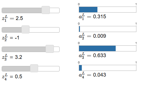
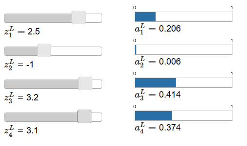
By increasing z ^L ₄ , one can observe an increase in the corresponding output activation, a ^L ₄ , and a decrease in the remaining output activations. Decreasing z ^L ₄ a ^L ₄ will decrease, and all other output activations will increase. Looking closely, you will see that in both cases, the total change in other activations accurately compensates for the change that occurs in a ^L ₄ . The reason for this is that there is a guarantee that all output activations total 1, which we can prove with the help of equation (78) and some algebra:

$$

$$\ sum_j a ^ L_j = \ frac {\ sum_j e ^ {z ^ L_j}} {\ sum_k e ^ {z ^ L_k}} = 1 \ tag {79}$$

As a result, with an increase in a ^L _{4, the} remaining output activations must decrease by the same amount in total to ensure that the sum of all output activations will be 1. And, of course, similar statements will be true for all other activations.

From equation (78) it also follows that all output activations are positive, since the exponential function is positive. Combining this with the observation from the previous paragraph, we obtain that the output of the Softmax layer will be a set of positive numbers, giving a total of 1. In other words, the output of the Softmax layer can be represented as a probability distribution.

The fact that the output of the Softmax layer is a probability distribution is very nice. In many problems, it is convenient to be able to interpret the output activations a ^L _j as an estimate by the network of the probability that the correct variant is j. So, for example, in the classification problem MNIST, we can interpret a ^L _j as an estimate by the network of the probability that _j is the correct way to classify a digit.

Conversely, if the output layer was sigmoid, then we definitely cannot assume that the activations form the probability distribution. I will not prove this strictly, but it is reasonable to assume that sigmoid activations in the general case do not form a probability distribution. Therefore, using a sigmoid output layer, we will not get such a simple interpretation of output activations.

Exercise

• Create an example showing that on a network with a sigmoid output layer, the output activations a ^L _j do not always add up to 1.

We are starting to understand a bit about Softmax functions and how Softmax layers behave. Just to sum up the intermediate result: the exponents in equation (78) guarantee that all output activations will be positive. The sum in the denominator of equation (78) ensures that the Softmax output will total 1. Therefore, this kind of equation does not seem mysterious anymore: this is a natural way to ensure that the output activations form a probability distribution. Softmax can be imagined as a method of zooming z ^L _j and then compressing them into a handful to form a probability distribution.

Exercises

• Softmax monotonicity. Show that ∂a ^L _j / ∂z ^L _{k is} positive if j = k, and negative if j ≠ k. As a consequence, an increase in z ^L _{j is} guaranteed to increase the corresponding output activation a ^L _j , and reduce all other output activations. We have already seen this empirically using the sliders, but this proof will be rigorous.
• Softmax nonlocality. A nice feature of sigmoid layers is that the output a ^L _j is a function of the corresponding weighted input, a ^L _j = σ (z ^L _j ). Explain why this is not so with the Softmax layer: any output activation a ^L _j depends on all weighted inputs.

Task

• Invert Softmax layer. Suppose we have an NA with an output Softmax layer and the activations a ^L _{j are} known. Show that the corresponding weighted inputs are of the form z ^L _j = ln a ^L _j + C, where C is a constant independent of j.

The problem of slowing down learning

We already got acquainted with Softmax-layers of neurons. But so far we have not seen how Softmax layers allow us to solve the problem of slowing learning. To understand this, let's define a log-likelihood cost function. We will use x to denote the network learning input, and y for the corresponding desired output. Then the LPS associated with this learning entry will be:

$$

$$C \ equiv - \ ln a ^ L_y \ tag {80}$$

So, if, for example, we are trained in MNIST images, and image 7 is sent to the input, then LPS will be equal to −ln a ^L ₇ . To understand this intuitively, consider the case when the network copes well with recognition, that is, it is sure that it is at input 7. In this case, it will estimate the value of the corresponding probability a ^L ₇ as close to 1, therefore the cost −ln a ^L ₇ will be small . Conversely, if the network works poorly, then the probability of a ^L ₇ will be less, and the cost −ln a ^L ₇ will be more. Therefore, LPS behaves as you would expect from a cost function.

What about the problem of slowing down learning? To analyze it, we recall that the main thing in slowing down is the behavior of ∂C / ∂w ^L _jk and ∂C / ∂ b ^L _j . I will not describe in detail the taking of the derivative - I will ask you to do it in problems, but using some kind of algebra it can be shown that:

$$

$$\ frac {\ partial C} {\ partial b ^ L_j} = a ^ L_j-y_j \ tag {81}$$

$$

$$\ frac {\ partial C} {\ partial w ^ L_ {jk}} = a ^ {L-1} _k (a ^ L_j-y_j) \ tag {82}$$

I played a little with the notation here, and use “y” a little bit differently than in the last paragraph. There, y meant the desired output of the network - that is, if the output is “7”, then the input was image 7. And in these equations, y denotes the vector of output activations corresponding to 7, that is, a vector that has all zeros except one in 7 th position.

These equations are the same as the similar expressions obtained by us in an earlier analysis of cross entropy. Compare, for example, equations (82) and (67). This is the same equation, although in the latter one averaged over the teaching examples. And, as in the first case, these expressions guarantee the absence of a slowdown in learning. It is useful to imagine that the output Softmax-layer with LPS is quite similar to the layer with a sigmoid output and cost based on cross-entropy.

Given their similarity, what should I use - sigmoid output and cross-entropy, or Softmax-output and LPS? In fact, in many cases both approaches work well. Although later in this chapter we will use a sigmoid output layer with a value based on cross-entropy. Later in chapter 6, we will sometimes use Softmax-exit and LPS. The reason for the change is to make some of the following networks more similar to the networks found in some influential research papers. From a more general point of view, Softmax and LPS should be used when you need to interpret the output activation as probabilities. This is not always necessary, but it may be useful in classification problems (such as MNIST), which include non-overlapping classes.

Tasks

• Derive the equations (81) and (82).
• Where did the name Softmax come from? Suppose we change the Softmax function so that the output activations are given by the equation

  $$

  $$a ^ L_j = \ frac {e ^ {c z ^ L_j}} {\ sum_k e ^ {c z ^ L_k}} \ tag {83}$$
  where c is a positive constant. Note that c = 1 corresponds to the standard Softmax-function. But using a different value of c, we get another function that will still be qualitatively similar to Softmax. Show that the output activations form a probability distribution, as is the case with the usual Softmax. Suppose we make c very large, that is, c → & inf ;. What is the limiting value of output activations a ^L _j ? After solving this problem, it should be clear why a function with c = 1 is considered a “softened version” of the maximum function. Hence the term softmax.
• Reverse distribution with Softmax and LPS. In the last chapter, we derived a back distribution algorithm for a network containing sigmoid layers. To apply this algorithm to the network and Softmax layers, we need to derive an expression for the error δ ^L _j ≡ ∂C / ∂z ^L _j . Show that the appropriate expression would be

  $$

  $$\ delta ^ L_j = a ^ L_j -y_j \ tag {84}$$
  Using this expression, we can apply the back-propagation algorithm to the network using the output Softmax-layer and LPS.

Retraining and regularization

The Nobel laureate Enrico Fermi was somehow asked for an opinion on the mathematical model proposed by several colleagues to solve an important unsolved physical problem. The model fit the experiment perfectly, but Fermi was skeptical. He asked how many free parameters in it can be changed. “Four,” he was told. Fermi replied: "I remember how my friend Johnny von Neumann liked to say that with four parameters you can shove an elephant there, and with five you can make him wave his trunk."

The meaning of the story, of course, is that models with a large number of free parameters can describe a surprisingly wide range of phenomena.Even if such a model works well with the available data, it does not automatically make it a good model. It simply may mean that the model has enough freedom so that it can describe almost any set of data of a given size without revealing the main idea of ​​the phenomenon. When this happens, the model works well with existing data, but will not be able to generalize the new situation. The true test of the model is its ability to make predictions in situations that it has not previously encountered.

Fermi and von Neumann were suspicious of models with four parameters. Our NA with 30 hidden neurons for classifying MNIST numbers has almost 24,000 parameters! These are quite a few parameters. Our NA with 100 hidden neurons has almost 80,000 parameters, and the advanced deep NA of these parameters sometimes have millions or even billions. Can we trust the results of their work?

Let's complicate this problem by creating a situation in which our network poorly generalizes a new situation for it. We will use NAs with 30 hidden neurons and 23,860 parameters. But we will not train the network with all 50,000 MNIST images. Instead, use only the first 1000. The use of a limited set will make the problem of generalization more obvious. We will learn as before using the cost function based on cross entropy, with a learning rate of η = 0.5 and a mini-package size of 10. However, we will study 400 epochs, which is slightly more than it was before, because of the teaching examples we don't have much. Let's use network2 to see how the cost function changes:

 >>> import mnist_loader >>> training_data, validation_data, test_data = \ ... mnist_loader.load_data_wrapper() >>> import network2 >>> net = network2.Network([784, 30, 10], cost=network2.CrossEntropyCost) >>> net.large_weight_initializer() >>> net.SGD(training_data[:1000], 400, 10, 0.5, evaluation_data=test_data, ... monitor_evaluation_accuracy=True, monitor_training_cost=True) 

Using the results, we can build a graph of the cost change when training the network (the graphs are made using the overfitting.py program):



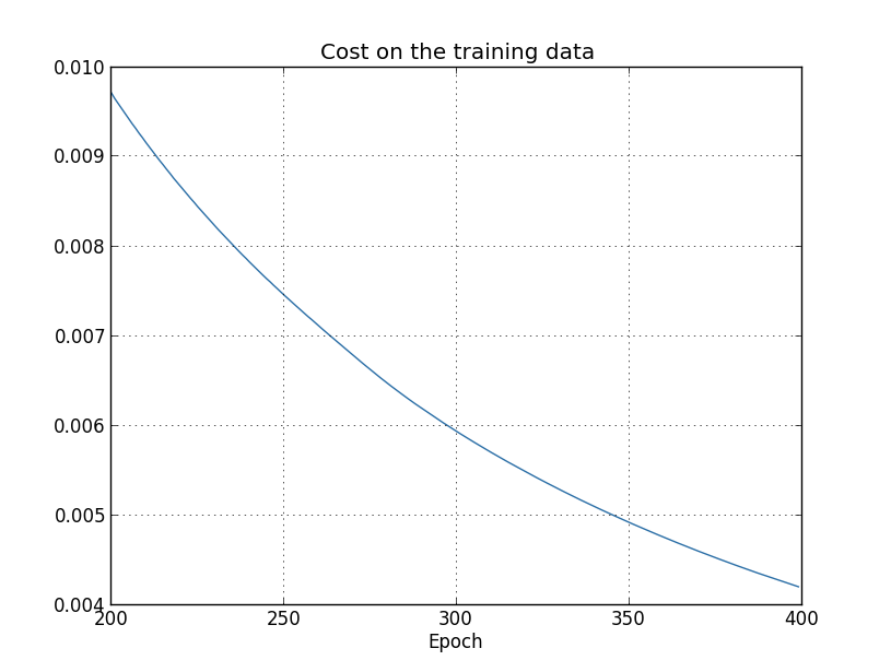
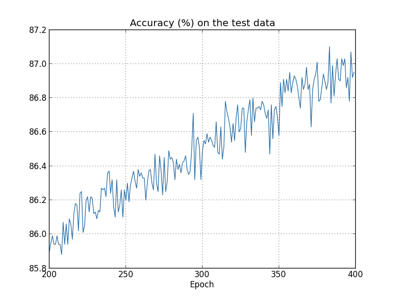
It looks encouraging, there is a smooth decrease in cost, as expected. Consider that I showed only the epochs from 200 to 399. As a result, we see on an enlarged scale the later stages of training, at which, as we will see later, all the most interesting things happen.

Now let's see how the classification accuracy of the test data changes over time:



Here I again increased the schedule. In the first 200 epochs that are not visible here, accuracy increases to almost 82%. Then learning gradually slows down. Finally, at about the 280th era, classification accuracy ceases to improve. In the later epochs, only small stochastic fluctuations are observed around the value of accuracy achieved at the 280th epoch. Compare this with the previous graph, where the cost associated with the training data gradually decreases. If you study only this value, it will seem that the model is improving. However, the results of the work with the verification data tell us that this improvement is only an illusion. As in the model that Fermi didn’t like, what our network studies after the 280th era is no longer generalized to verification data. Therefore, this training ceases to be useful. We say that after the 280th era, the network is being retrained,or overfitting or overtraining.

You may wonder if it is a problem that I study cost based on the training data, and not the accuracy of the classification of the verification data. In other words, perhaps the problem is that we compare apples with oranges. What will happen if we compare the cost of training data with the cost of verification, that is, we will compare comparable measures? Or perhaps we could compare the classification accuracy of both training and verification data? In fact, the same phenomenon occurs regardless of how the comparison is made. But the details are changing. For example, let's look at the cost of verification data:



It can be seen that the cost of the verification data improves to about the 15th era, and then begins to deteriorate altogether, although the cost of the training data continues to improve. This is another sign of the retrained model. However, the question arises, what era should we consider the point at which retraining begins to dominate training - 15 or 280? From a practical point of view, we are still interested in improving the accuracy of the classification of verification data, and cost is only an intermediary of classification accuracy. Therefore, it makes sense to consider the 280 era as a point after which retraining begins to dominate over the training of our NA.

Another sign of retraining can be seen in the accuracy of the classification of training data:



Accuracy increases, reaching 100%. That is, our network correctly classifies all 1000 training images! In the meantime, verification accuracy grows only to 82.27%. That is, our network only studies the features of the training set, and does not learn to recognize numbers at all. It seems that the network simply remembers the training set, not well enough understanding the numbers in order to generalize it to the test set.

Retraining is a serious problem with NA. This is especially true for modern NA, which usually have a huge amount of weights and offsets. For effective training, we need a way to determine when retraining occurs so as not to retrain. We would also like to be able to reduce the effects of retraining.

The obvious way to detect retraining is to use the approach above, to monitor the accuracy of working with the verification data in the network training process. If we see that the accuracy of the verification data is no longer improving, we must stop learning. Of course, strictly speaking, this will not necessarily be a sign of retraining. It is possible that the accuracy of work with verification and training data will stop improving simultaneously. Yet the use of such a strategy will prevent retraining.

And we will use a small variation of this strategy. Recall that when we load data into MNIST, we divide it into three sets:

 >>> import mnist_loader >>> training_data, validation_data, test_data = \ ... mnist_loader.load_data_wrapper() 

So far we have used training_data and test_data, and ignored validation_data [confirming]. The validation_data contains 10,000 images that differ from both the 50,000 images of the MNIST training set and the 10,000 images of the check set. Instead of using test_data to prevent retraining, we will use validation_data. For this we will use almost the same strategy that was described above for test_data. That is, we will calculate the accuracy of the classification of validation_data at the end of each epoch. As soon as the classification accuracy validation_data is saturated, we will stop learning. This strategy is called an early stop. Of course, in practice we will not be able to immediately find out that accuracy has been saturated. Instead, we will continue learning until we make sure of this (and decidewhen you need to stop is not always easy, and you can use more or less aggressive approaches for this).

Why use validation_data to prevent retraining, not test_data? This is part of a more general strategy — use validation_data to evaluate different choices for hyper-parameters — the number of epochs for training, the speed of learning, the best network architecture, etc. We use these estimates to find and assign good values ​​to hyperparameters. And although I haven’t mentioned it yet, it was partly because of this that I made the choice of hyperparameters in the early examples in the book.

Of course, this remark does not answer the question of why we use validation_data, rather than test_data, to prevent retraining. It simply replaces the answer to a more general question - why do we use validation_data, rather than test_data, to select hyper parameters? To understand this, keep in mind that when choosing hyper parameters we will most likely have to choose from a variety of their options. If we assign hyperparameters based on the ratings from test_data, we will probably fit this data too much under test_data. That is, we may find hyperparameters well suited to the specifics of specific data from test_data, but the operation of our network will not be generalized to other data sets. We avoid this by selecting hyper parameters with validation_data. And then, having received the GPs we need,we conduct a final accuracy assessment using test_data. This gives us confidence that our results of working with test_data are a true measure of the degree of generalization of the NA. In other words, supporting data is such special training data that helps us learn good GP. This approach to GP search is sometimes called the hold method, since validation_data is "held" separately from training_data.

In practice, even after assessing the quality of work on test_data, we will want to change our opinion and try a different approach — perhaps a different network architecture — that will include searching for a new set of GPs. In this case, will there be a danger that we will unnecessarily adapt to test_data? Do we need a potentially infinite number of data sets to make us sure that our results are well summarized? In general, this is a deep and complex problem. But for our practical purposes, we will not worry too much about this. We will simply dive headlong into further exploration using a simple retention method based on training_data, validation_data and test_data, as described above.

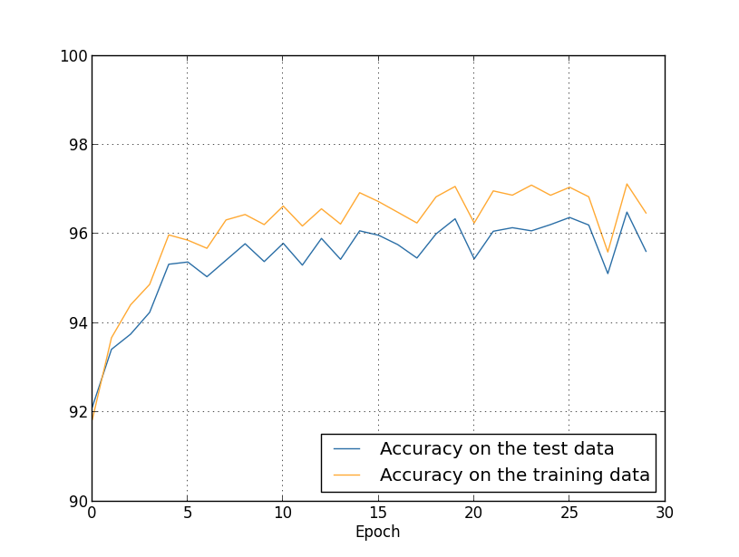
So far, we have considered retraining using 1000 training images. What happens if we use a complete training set of 50,000 images? We will leave all other parameters unchanged (30 hidden neurons, learning speed 0.5, mini-package size 10), but we will learn 30 epochs using all 50,000 images. Here is a graph showing the accuracy of the classification on the training and verification data. Note that here I used the test [test], rather than the validation data, to make the results easier to compare with earlier graphs.



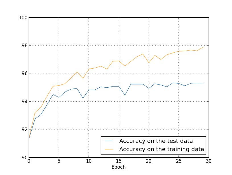
It can be seen that the accuracy indicators on the verification and training data remain closer to each other than when using 1000 training examples. In particular, the best classification accuracy, 97.86%, is only 2.53% higher than the 95.33% verification data. Compare with an early gap of 17.73%! Retraining occurs, but has greatly diminished. Our network summarizes information much better, moving from training to verification data. In general, one of the best ways to reduce retraining is to increase the amount of training data. Taking enough training data, it is difficult to retrain even a very large network. Unfortunately, it is expensive and / or difficult to obtain training data, so this option is not always practical.

Regularization

Increasing the amount of training data is one way to reduce retraining. Are there any other ways to reduce the manifestations of retraining? One possible approach is to reduce the size of the network. True, large networks have potentially more opportunities than small ones, therefore we reluctantly resort to this option.

Fortunately, there are other techniques that can reduce retraining, even when we have fixed the size of the network and training data. They are known as regularization techniques. In this chapter, I will describe one of the most popular techniques, sometimes called loosening weights, or L2 regularization. Her idea is to add an additional member to the cost function called a regularization member. Here is a cross-sectional entropy with regularization:

$$

$$C = -\frac{1}{n} \sum_{xj} \left[ y_j \ln a^L_j+(1-y_j) \ln (1-a^L_j)\right] + \frac{\lambda}{2n} \sum_w w^2 \tag{85}$$

The first term is a common expression for cross entropy. But we added the second one, namely, the sum of the squares of all weights of the network. It is scaled by the factor λ / 2n, where λ> 0 is the regularization parameter and n, as usual is the size of the training set. We will discuss how to choose λ. It is also worth noting that the regularization term does not include offsets. About this below.

Of course, it is possible to regularize other cost functions, for example, quadratic. This can be done in a similar way:

$$

$$C = \frac{1}{2n} \sum_x \|y-a^L\|^2 + \frac{\lambda}{2n} \sum_w w^2 \tag{86}$$

In both cases, you can write a regularized cost function, like

$$

$$C = C_0 + \frac{\lambda}{2n} \sum_w w^2 \tag{87}$$

where C ₀ is the original cost function without regularization.

It is intuitively clear that the meaning of regularization is to incline the network towards a preference for smaller weights, all other things being equal. Large weights will be possible only if they significantly improve the first part of the cost function. In other words, regularization is a way to choose a compromise between finding small weights and minimizing the original cost function. It is important that these two elements of a compromise depend on the value of λ: when λ is small, we prefer to minimize the original cost function, and when λ is large, we prefer small weights.

It’s not at all obvious why choosing such a compromise should help reduce overtraining! But it turns out helps. We will understand why it helps, in the next section. But first, let's work with an example showing that regularization really reduces retraining.

To construct an example, we first need to understand how to apply a learning algorithm with a stochastic gradient descent to a regularized NA. In particular, we need to know how to calculate the partial derivatives, ∂C / ∂w and ∂C / ∂b for all weights and offsets in the network. After taking the partial derivatives in equation (87), we get:

$$

$$\frac{\partial C}{\partial w} = \frac{\partial C_0}{\partial w} + \frac{\lambda}{n} w \tag{88}$$

$$

$$\frac{\partial C}{\partial b} = \frac{\partial C_0}{\partial b} \tag{89}$$

The terms 0C ₀ / ∂w and ∂C ₀ / ∂w can be calculated through the PR, as described in the previous chapter. We see that it is easy to calculate the gradient of the regularized cost function: it is just necessary, as usual, to use the OR, and then add λ / nw to the partial derivative of all weight terms. The partial derivatives with respect to displacements do not change, therefore the rule of learning by gradient descent for displacements does not differ from the usual:

$$

$$b \rightarrow b -\eta \frac{\partial C_0}{\partial b} \tag{90}$$

The learning rule for weights turns into:

$$

$$w \rightarrow w-\eta \frac{\partial C_0}{\partial w}-\frac{\eta \lambda}{n} w \tag{91}$$

$$

$$= \left(1-\frac{\eta \lambda}{n}\right) w -\eta \frac{\partial C_0}{\partial w} \tag{92}$$

Everything is the same as in the usual rule of gradient descent, except that we first scale the weight w by a factor 1 - ηλ / n. This scaling is sometimes called loosening the scale because it reduces the weight. At first, it seems that weights uncontrollably tend to zero. But this is not the case, since the other term can lead to an increase in weights, if it leads to a decrease in the irregular cost function.

Well, let gradient descent work like this. What about stochastic gradient descent? Well, as in the irregularized version of the stochastic gradient descent, we can estimate ∂C ₀ / ∂w by averaging over the mini-packet m training examples. Therefore, the regularized learning rule for stochastic gradient descent turns into (see equation (20)):

$$

$$w \rightarrow \left(1-\frac{\eta \lambda}{n}\right) w -\frac{\eta}{m} \sum_x \frac{\partial C_x}{\partial w} \tag{93}$$

where the sum goes according to the teaching examples x in the mini-package, and C _x - the irregular cost for each teaching example. Everything is the same as in the usual rule of stochastic gradient descent, with the exception of 1 - ηλ / n, the weight reduction factor. Finally, for completeness, let us write down a regularized rule for offsets. Naturally, it is exactly the same as in the unregularized case (see equation (21)):

$$

$$b \rightarrow b - \frac{\eta}{m} \sum_x \frac{\partial C_x}{\partial b} \tag{94}$$

where the sum goes according to the teaching examples x in the mini-package.

Let's see how regularization changes the effectiveness of our NA. We will use a network with 30 hidden neurons, a mini-packet of size 10, a learning rate of 0.5, and a cost function with cross-entropy. However, this time we will use the regularization parameter λ = 0.1. In the code, I called this variable lmbda, because the word lambda is reserved in python for things unrelated to our theme. I also used test_data again instead of validation_data. But I decided to use test_data, since the results can be compared directly with our early, irregularized results. You can easily change the code so that it uses validation_data, and make sure that the results are similar.

 >>> import mnist_loader >>> training_data, validation_data, test_data = \ ... mnist_loader.load_data_wrapper() >>> import network2 >>> net = network2.Network([784, 30, 10], cost=network2.CrossEntropyCost) >>> net.large_weight_initializer() >>> net.SGD(training_data[:1000], 400, 10, 0.5, ... evaluation_data=test_data, lmbda = 0.1, ... monitor_evaluation_cost=True, monitor_evaluation_accuracy=True, ... monitor_training_cost=True, monitor_training_accuracy=True) 

The cost of training data is constantly decreasing, as in the earlier case, without regularization:



But this time, the accuracy on test_data continues to increase during all 400 epochs:



Obviously, regularization suppressed retraining. Moreover, the accuracy has increased significantly, and the peak classification accuracy reaches 87.1%, compared with the peak of 82.27% achieved in the case of non-regularization. And in general, we almost certainly achieve the best results, continuing our training after 400 ages. Apparently, empirically, regularization makes our network better summarize knowledge, and significantly reduces the effects of retraining.

What happens if we leave our artificial environment, which uses only 1,000 training images, and return to the full set of 50,000 images? Of course, we have already seen that retraining presents a far less serious problem with a full set of 50,000 images. Does regularization help improve the result? Let's keep the previous values ​​of the hyperparameters - 30 epochs, speed 0.5, mini-packet size 10. However, we need to change the regularization parameter. The fact is that the size n of the training set jumped from 1000 to 50 000, and this changes the factor of weakening the weights 1 - ηλ / n. If we continue to use λ = 0.1, this would mean that the weights are weakened much less, and as a result, the effect of regularization decreases. We compensate for this by adopting λ = 5.0.

Well, let's train our network by re-initializing the weights first:

 >>> net.large_weight_initializer() >>> net.SGD(training_data, 30, 10, 0.5, ... evaluation_data=test_data, lmbda = 5.0, ... monitor_evaluation_accuracy=True, monitor_training_accuracy=True) 

We get the results:



A lot of everything pleasant. First, our classification accuracy on verification data has grown, from 95.49% without regularization to 96.49% with regularization. This is a major improvement. Secondly, it can be seen that the gap between the results of work on the training and test sets is much lower than before, less than 1%. The gap is still decent, but we have obviously made significant progress in reducing retraining.

Finally, see what kind of classification accuracy we will get when using 100 hidden neurons and the regularization parameter & lambda = 5.0. I will not give a detailed analysis of retraining, this is done just for the sake of interest, to see how much accuracy can be achieved with our new tricks: the cost function with cross entropy and L2 regularization.

 >>> net = network2.Network([784, 100, 10], cost=network2.CrossEntropyCost) >>> net.large_weight_initializer() >>> net.SGD(training_data, 30, 10, 0.5, lmbda=5.0, ... evaluation_data=validation_data, ... monitor_evaluation_accuracy=True) 

The end result is a classification accuracy of 97.92% on supporting data. Big jump in comparison with the case with 30 hidden neurons. You can adjust a little more, start the process for 60 epochs with η = 0.1 and λ = 5.0, and overcome the barrier of 98%, reaching an accuracy of 98.04 on supporting data. Not bad for 152 lines of code!

I described regularization as a way to reduce retraining and increase classification accuracy. But these are not its only advantages. Empirically, having tried our MNIST network through many launches, changing weights each time, I found that launches without regularization sometimes “stuck”, obviously, hitting the local minimum of the cost function. As a result, different launches sometimes gave very different results. Regularization, on the contrary, makes it possible to obtain reproducible results much easier.

Why is this so?Heuristically, when the cost function does not have a regularization, the length of the weight vector is likely to grow, all other things being equal. Over time, this can lead to a very large vector of scales. And because of this, the weights vector can get stuck, showing approximately in the same direction, since changes due to gradient descent make only tiny changes in the direction when the vector is long. I believe that because of this phenomenon, our learning algorithm is very difficult to study the weights space, and therefore it is difficult to find a good minimum of the cost function.