Deep (Learning + Random) Forest and parsing articles

We continue to talk about the conference on statistics and machine learning AISTATS 2019. In this post we will discuss articles about deep models from tree ensembles, mix regularization for highly sparse data and time-effective approximation of cross-validation.

Deep Forest Algorithm: An Exploration to Non-NN Deep Models based on Non-Differentiable Modules

Zhi-Hua Zhou (Nanjing University)
→ Presentation
→ Article
Implementations - below

A professor from China spoke about the tree ensemble, which the authors call the first in-depth training on non-differentiable modules. This may seem too loud a statement, but this professor and his H-index 95 are invited speakers, this fact makes it possible to take the statement more seriously. The basic theory of Deep Forest has been developed a long time ago, the original article was already in 2017 (almost 200 citations), but the authors write libraries and improve the speed algorithm every year. And now, it seems, they have reached the level when this beautiful theory can finally be applied in practice.

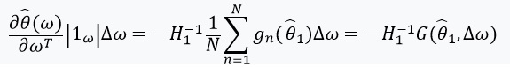
General view of the Deep Forest architecture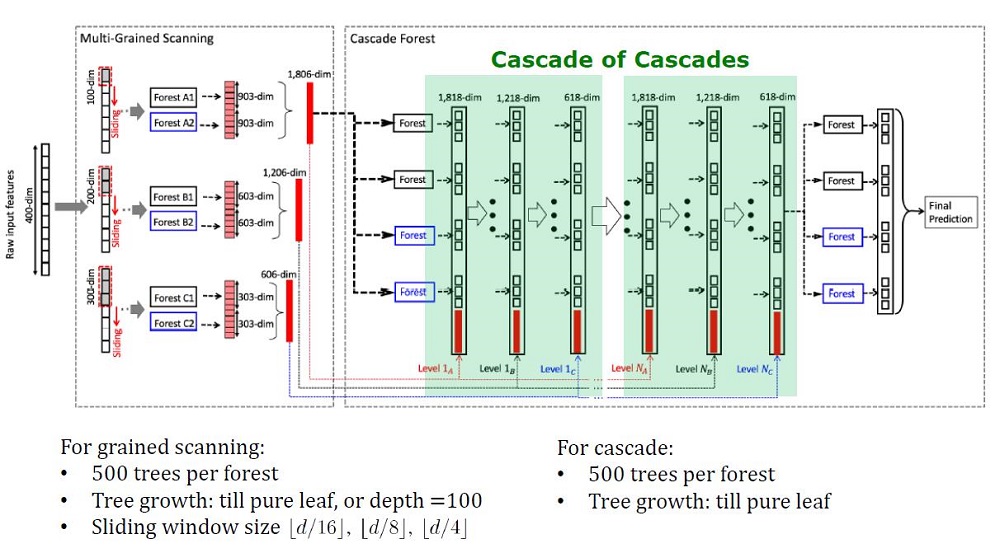

Prerequisites

Deep models, which now mean deep neural networks, are used to capture complex dependencies in data. Moreover, it turned out that increasing the number of layers is more efficient than increasing the number of units on each layer. But neural networks have their disadvantages:

It takes a lot of data to not retrain,
It takes a lot of computing resources to learn in a reasonable time.
Too many hyperparameters that are difficult to configure optimally.

In addition, elements of deep neural networks are differentiable modules that are not necessarily effective for each task. Despite the complexity of neural networks, conceptually simple algorithms, like a random forest, often work better or not much worse. But for such algorithms you need to manually construct features, which is also difficult to do optimally.

Already, researchers have noticed that the ensembles at Kaggle: "very poverfull to do the practice", and inspired by the words of Scholl and Hinton about the fact that differentiation is the weakest side of Deep Learning, they decided to create an ensemble of trees with DL properties.

Slide “How to make a good ensemble”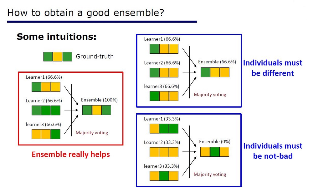

The architecture was derived from the properties of the ensembles: the elements of the ensembles should not be very poor in quality and different.

GcForest consists of two stages: Cascade Forest and Multi-Grained Scanning. Moreover, so that the cascade is not retrained, it consists of 2 types of trees - one of which is absolutely random trees that can be used on unpartitioned data. The number of layers is determined within the algorithm by cross-validation.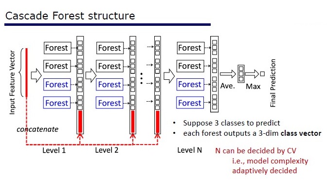

Two types of trees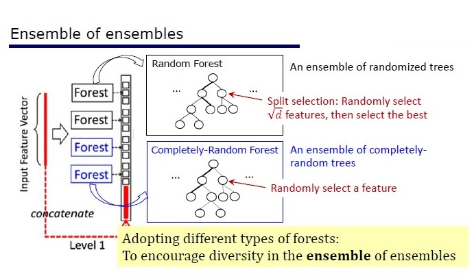

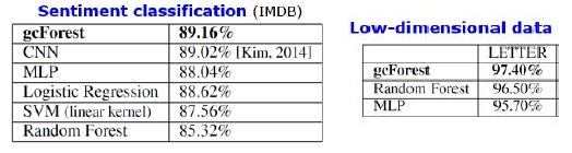
results

In addition to the results on standard datasets, the authors tried to apply gcForest on transactions of the Chinese payment system for fraud searches and got F1 and AUC much higher than those of LR and DNN. These results are only in the presentation, but the code to run on some standard datasets is on Git.

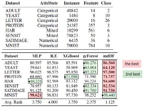
Shutter Algorithm Results. mdDF is optimal Margin Distribution Deep Forest, a variant of gcForest

Pros:

Few hyperparameters, the number of layers is configured automatically within the algorithm.
Default options are set to work well on many tasks.
Adaptive complexity of the model, on small data - a small model
No need to set features
It works in comparable quality with deep neural networks, and sometimes better

Minuses:

Not accelerated on the GPU
In the pictures plays DNNs

Neural grids have a gradient damping problem, and deep woods have a problem of “diversity vanishing”. Since this is an ensemble, the more “different” and “good” elements to use - the higher the quality. The problem is that the authors have already reviewed almost all the classical approaches (sampling, randomization). Until new fundamental research appears in the “differences” topic, it will be difficult to improve the quality of deep forest. But now it is possible to improve the speed of calculations.

Reproducible results

XGBoost won such a cool gain on the tabular data, and wanted to reproduce the result. I took Adults datasets and applied GcForestCS (slightly accelerated version of GcForest) with parameters from the authors of the article and XGBoost with default parameters. In the example that the authors had, the categorical features were already pre-processed somehow, but not how. In the end, I used CatBoostEncoder and another metric - ROC AUC. The results were statistically different - XGBoost won. The running time of XGBoost is insignificant, and for gcForestCS - 20 minutes each, each cross-validation on 5 folds. On the other hand, the authors tested the algorithm on different datasets, and the parameters for this dataset were adjusted to their pre-processing features.

Code can be found here .

Implementations

→ Official code from the authors of the article
→ Official improved version, works faster, but there is no documentation
→ Implementation easier

PcLasso: the lasso meets principal components regression

J. Kenneth Tay, Jerome Friedman, Robert Tibshirani (Stanford University)

→ Article
→ Presentation
→ Example of use

In early 2019, J. Kenneth Tay, Jerome Friedman and Robert Tibshirani from Stanford University proposed a new method of teaching with a teacher, especially suitable for sparse data.

The authors of the article solved the problem of analyzing data on the study of gene expression, which are described in Zeng & Breesy (2016). Target is the mutational status of the p53 gene, which regulates gene expression in response to various cellular stress signals. The aim of the study is to identify predictors that correlate with the mutational status of p53. The data consists of 50 lines, 17 of which are classified as normal and the remaining 33 are mutations in the p53 gene. In accordance with the analysis in Subramanian et al. (2005) 308 sets of genes that are between 15 and 500 are included in this analysis. These gene kits contain a total of 4301 genes and are available in the grpregOverlap R package. When expanding data to handle overlapping groups, 13,237 columns go out. The authors of the article applied the pcLasso method, which helped to improve the model results.

In the picture we see an increase in AUC when using “pcLasso”

The essence of the method

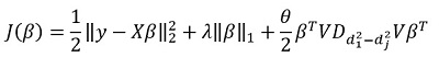
Method combines l_1 -regularization with l_2 , which narrows the vector of coefficients to the main components of the matrix of features. They called the proposed method "lasso core components" ("pcLasso" available on R). The method can be especially powerful if the variables are pre-grouped (the user chooses what and how to group). In this case, pcLasso compresses each group and gets a solution in the direction of the main components of this group. In the process of decision, the selection of significant groups among the existing ones is also performed.

We present the diagonal matrix of the singular decomposition of a centered matrix of attributes in the following way:

Our singular decomposition of the centered matrix X (SVD) is represented as X = UDV ^ T where - diagonal matrix consisting of singular values. In this form l_2 -regularization can be represented:
$\ beta ^ T VZV ^ T \ beta$ Where - diagonal matrix containing the function of the squares of singular values: $Z_ {11} = f_1 (d_1 ^ 2, d_2 ^ 2, ..., d_m ^ 2), ..., Z_ {22} = f_2 (d_1 ^ 2, d_2 ^ 2, ..., d_m ^ 2)$ .

In general, in l_2 -regularization $Z_ {jj} = 1$ for all that matches $\ beta ^ T \ beta$ . They propose to minimize the following functionality:

Here - matrix of differences of diagonal elements d_1 ^ 2-d_1 ^ 2, d_1 ^ 2-d_2 ^ 2, ..., d_1 ^ 2-d_m ^ 2 . In other words, we control the vector. $\ beta$ also with the help of the hyperparameter $\ theta$ .
Transforming this expression, we get the solution:

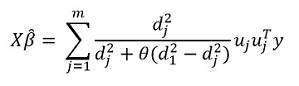
But the main "feature" of the method, of course, is the ability to group data, and based on these groups, select the main components of the group. Then we rewrite our solution in the form:

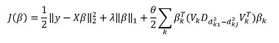
Here $\ beta_k$ - vector subvector $\ beta$ corresponding to group k, $d_k = (d_ {k1}, ..., d_ {kmk})$ - singular values X_k arranged in descending order, and $D_ {d_ {k1} ^ 2-d_ {kj} ^ 2}$ - diagonal matrix $d_ {k1} ^ 2-d_ {kj} ^ 2, j = 1,2, ..., m_k$

Some comments on the solution of the target functional:

The objective function is convex, and the non-smooth component is separable. Consequently, it can be effectively optimized using gradient descent.
The approach is to fix multiple values. $\ theta$ (including zero, respectively, getting the standard -regularization), and then optimize: picking up $\ lambda$ . Accordingly, the parameters $\ theta$ and $\ lambda$ are selected for cross-validation.
Parameter $\ theta$ hard to interpret. In the software (package "pcLasso"), the user himself sets the value of this parameter, which belongs to the interval [0,1], where 1 corresponds to $\ theta$ = 0 (lasso).

In practice, varying the values $\ theta$ = 0.25, 0.5, 0.75, 0.9, 0.95, and 1, you can cover a large range of models.

The algorithm itself is as follows

This algorithm is already written in R, if you wish, you can already use it. The library is called 'pcLasso'.

A Swiss Army Infinitesimal Jackknife

Ryan Giordano (UC Berkeley); William Stephenson (MIT); Runjing Liu (UC Berkeley);
Michael Jordan (UC Berkeley); Tamara Broderick (MIT)

→ Article
→ Code

The quality of machine learning algorithms is often evaluated by multiple cross-validation (cross-validation or bootstrap). These methods are powerful, but slow on large data sets.

In this paper, colleagues use linear approximation of scales, producing results that work faster. This linear approximation is known in the statistical literature as the “infinitesimal jackknife”. It is mainly used as a theoretical tool for proving asymptotic results. The results of the paper are applicable regardless of whether the weights and data are stochastic or deterministic. As a consequence, this approximation consistently evaluates the true cross-validation for any fixed k.

Handing Paper Award to the author of the article

The essence of the method

Consider the problem of estimating an unknown parameter. $\ theta \ in \ Omega _ {\ theta} \ subset R ^ {D}$ where $\ Omega _ {\ theta}$ - compact, and the size of our dataset - . Our analysis will be conducted on a fixed set of data. We define our assessment $\ theta \ in \ Omega _ {\ theta}$ in the following way:

For each let's set ( $\ theta$ ) - function from $\ Omega _ {\ theta} \ subset R ^ {D}$
$\ omega_n$ - a real number, and $\ omega$ - vector consisting of $\ omega_n$

Then $\ hat {\ theta}$ can be represented as:

Solving this optimization problem using the gradient method, we assume that the functions are differentiable and we can calculate the Hessian. The main problem that we solve is the computational costs associated with the assessment $\ hat {\ theta} ̂ (\ omega)$ for all $\ omega∈W$ . The main contribution of the authors of the article is to calculate the estimate $\ hat {\ theta} _1 = \ hat {\ theta} _1 (1 _ {\ omega})$ where $1_ \ omega = (1,1, ..., 1)$ . In other words, our optimization will depend only on derivatives $g_n (\ theta)$ , which we assume exist, and are the Hessian:

Next, we define an equation with a fixed point and its derivative: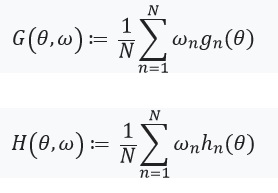

It is worth noting here that $G (\ theta ̂ (\ omega), w) = 0$ , because $\ hat {\ theta} (\ omega)$ - solution for $\ frac {1} {N} \ sum_ {n = 1} ^ {N} \ omega_n g_n (\ theta) = 0$ . Also define: $H_1 = H (\ hat {\ theta} _1,1_ \ omega)$ and matrix weights like: $\ Delta \ omega = \ omega-1_ \ omega \ in R ^ {n}$ . In that case, when H_1 has an inverse matrix, we can use the implicit function theorem and the 'chain rule':

This derivative allows us to form a linear approximation $\ hat {\ theta} ̂ (\ omega)$ through $\ hat {\ theta} _1$ which looks like this:

Because $\ hat {\ theta} _ {IJ}$ depends only on $\ hat {\ theta} _1$ and $\ Delta \ omega$ and not on solutions for any other values. $\ omega$ , accordingly, there is no need to recalculate anew and find new values of ω. Instead, the SLN (system of linear equations) must be solved.

results

In practice, this significantly reduces the time compared to cross-validation: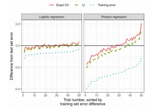

Source: https://habr.com/ru/post/458388/

All Articles

Deep (Learning + Random) Forest and parsing articles

Deep Forest Algorithm: An Exploration to Non-NN Deep Models based on Non-Differentiable Modules

PcLasso: the lasso meets principal components regression

A Swiss Army Infinitesimal Jackknife

More articles: