Mathematical model of a radio telescope with a super-long base

Introduction

One of the first radio telescopes was built by the American Grotto Reber in 1937. The radio telescope was a tin mirror with a diameter of 9.5 m mounted on a wooden frame:

By 1944, Reber compiled the first map of the distribution of cosmic radio waves in the Milky Way region.
')
The development of radio astronomy entailed a number of discoveries: in 1946, radio emission from the constellation Cygnus was discovered, in 1951 - extragalactic radiation, in 1963 - quasars, in 1965 open-relic background radiation at 7.5 cm wave.

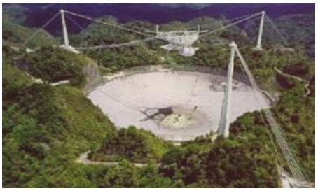
In 1963, a unique 300-meter radio telescope was built in Arecibo (Puerto Rico). This is a fixed bowl with a moving feed, built in the natural cleft of the area.

Single radio telescopes have a small angular resolution, which is determined by the formula:

T h e t a = f r a c l a m b d a d

$\ Theta = \ frac {\ lambda} {d}$
Where

l a m b d a

$\ lambda$ - wavelength,

d

$d$ - diameter of the radio telescope.

Obviously, to improve the resolution, it is necessary to increase the diameter of the antenna, which is physically a difficult task to accomplish. It was possible to solve it with the advent of radio interferometers.

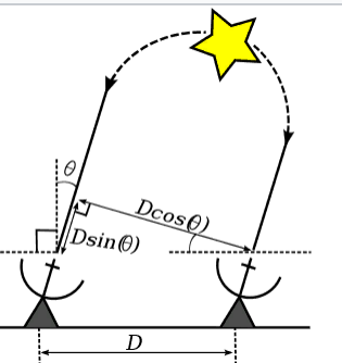
The front of an electromagnetic wave emitted by a distant star near the Earth can be considered flat. In the case of the simplest interferometer consisting of two antennas, the path difference of the rays that came to these two antennas will be equal to:

D e l t a = D c d o t s i n (T h e t a)

$\ Delta = D \ cdot sin (\ Theta)$ ,
Where:

D e l t a

$\ Delta$ - the path difference of the rays;

D

$D$ - the distance between the antennas;

T h e t a

$\ Theta$ - the angle between the direction of arrival of the rays and the normal to the line on which the antennas are located.

With

T h e t a = 0

$\ Theta = 0$ the waves arriving at both antennas are summed in phase. In antiphase the waves will be the first time when:

D e l t a = f r a c l a m b d a 2, T h e t a = a r c s i n f r a c l a m b d a 2 D

$\ Delta = \ frac {\ lambda} {2}, \ Theta = arcsin \ frac {\ lambda} {2D}$ ,
Where:

l a m b d a

$\ lambda$ - wavelength.

The next maximum will be at

D e l t a = l a m b d a,

$\ Delta = \ lambda,$ at least

D e l t a = f r a c 3 l a m b d a 2

$\ Delta = \ frac {3 \ lambda} {2}$ etc. A multi-petal radiation pattern (DN) is obtained, the width of the main lobe of which is

l a m b d a << D

$\ lambda << D$ equals

l a m b d a / D

$\ lambda / D$ . The width of the main lobe is determined by the maximum angular resolution of the radio interferometer, it is approximately equal to the width of the lobe.

Superlong-base radio interferometry (VLBI) is a type of interferometry used in radio astronomy, in which the receiving elements of the interferometer (telescopes) are located no closer than at continental distances from each other.

The VLBI method allows one to combine observations made by several telescopes, and thereby simulate a telescope whose dimensions are equal to the maximum distance between the original telescopes. The angular resolution of VLBI is tens of thousands of times greater than the resolving power of the best optical instruments.

Current state of VLBI - networks

Today, several VLBI networks listen to space:

European –EVN (European VLBI Network), consisting of more than 20 radio telescopes;
The American –VLBA (Very Long Baseline Array), which includes ten telescopes with a diameter of 25 meters each;
Japanese - JVN (Japanese VLBI Network) consists of ten antennas located in Japan, including four astrometric antennas (VERA project - VLBI Exploration of Radio Astrometry);
Australian - LBA (Long Baseline Array);
Chinese - CVN (Chinese VLBI Network), consisting of four antennas;
South Korean - KVN (Korean VLBI Network), which includes three 21-meter radio telescope;
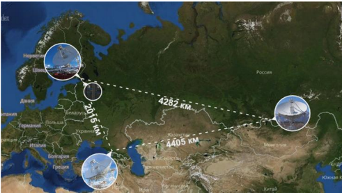
The Russian - based on the permanently operating radio-interferometric complex - “Quasar-KVO” with radio telescopes with a mirror diameter of 32 m, equipped with highly sensitive cryoreradiometers in the wavelength range from 1.35 cm to 21 cm. The length of the bases - the effective diameter of the synthesized “mirror” - is about 4400 km in the direction east-west (see drawing).

In VLBI - the Quasar-KVO complex, hydrogen standards are used as a reference frequency source for all frequency transformations, which use a transition between the levels of the hyperfine structure of the ground state of a hydrogen atom with a frequency of 1420.405 MHz, the corresponding line in radio astronomy 21 cm.

Tasks solved by means of VLBI

Astrophysics. The construction of radio images of natural space objects (quasars and other objects) with the resolution of the tenth and hundredths of mas (milliseconds of arc) is carried out.
Astrometric studies. The construction of coordinate systems. The objects of research are radio sources of extremely small angular sizes, including quasi-stellar radio sources and the nuclei of radio galaxies, which, due to their large distance, are almost ideal objects for creating a network of supporting fixed objects.
Studies on the celestial mechanics and dynamics of the solar system, space navigation. The establishment of a radio beacon on the surfaces of the planets and the tracking of the radio beacons of interplanetary automated stations allows using the VLBI method to study parameters such as the orbital motion of the planet, the direction of the axes of rotation and their precession, the dynamics of the satellite planet system. For the moon, the very important task of determining physical libration and determining the dynamics of the Moon-Earth systems is also solved.

Navigation in space by means of VLBI

Control of astronaut movements on the lunar surface in 1971. They moved with the help of the Rover lunar rover. The accuracy of determining its position relative to the lunar module reached 20 cm and depended mainly on the libration of the moon (Libration — periodic pendulum-like oscillations of the Moon relative to its center of mass);
Navigation support of delivery and discharge of balloon probes from flying vehicles into the atmosphere of Venus (VEGA project). The distance to Venus is more than 100 million km, the power of the transmitters is only 1 W. The launches of VEGA-1/2 vehicles took place in December 1984. The aerostats were released into the atmosphere of Venus on June 11 and 15, 1985. Observation was conducted for 46 hours.

Block diagram of a simplified VLBI - network

Based on a real VLBI network, using the Python software, we will model a simplified VLBB system as separate models for each block or process. This set of models will be enough to observe the basic processes. The block diagram of a simplified VLBI network is shown in the figure:

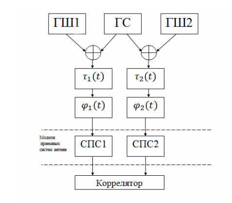
The system includes the following components:

the generator of the useful phase-modulated signal (HS);
noise generators (GSH1, GSH2). The system has two radio telescopes (receiving antennas), which have their own noise. In addition, there are noises from the atmosphere and other natural and artificial sources of radio emission;
a time delay unit that simulates a time-varying delay due to the rotation of the Earth;
phase shifter, modeling Doppler effect;
a signal conversion system (PCA), consisting of a local oscillator, for carrying the signal down in frequency, and a band-pass filter;
FX correlator.

The correlator circuit is shown in the following figure:

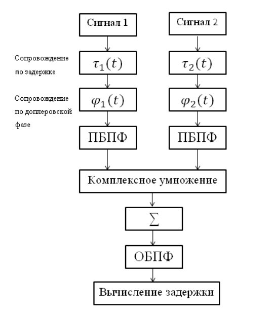
The given correlator circuit, which includes the following blocks:

forward fast Fourier transform (PBPF) and inverse Fourier transform (OBPF);
compensating for the previously introduced delay;
Doppler compensating effect;
complex multiplication of two spectra;
summation of accumulated realizations.

Navigation Signal Model

The most convenient for VLBI measurements are the navigation signals of satellite-based satellite navigation systems, such as GPS and GLONASS. There are a number of requirements for navigation signals:

allow well define pseudorange;
transmit information about the position of the navigation system;
be distinguishable from signals of other NA;
Do not interfere with other radio systems;
do not require to receive and transmit complex equipment.

The signal with binary (two-position) phase modulation - BPSK (binary phase shift key), which in the Russian-language literature is designated FM-2, satisfies them to a sufficient extent. This modulation changes the phase of the carrier wave, by π, which can be represented as:

S (t) = A c d o t G (t) c d o t c o s (2 p i f t),

$S (t) = A \ cdot G (t) \ cdot cos (2 \ pi ft),$

where G (t) is the modulating function.

To implement phase modulation, you can use two generators, each of which forms the same frequency, but with a different initial phase. The modulating function allows you to expand the signal spectrum and accurately measure the pseudorange (the distance between the satellite and the receiver, calculated from the signal propagation time without a correction for the difference between the satellite clock and the receiver).

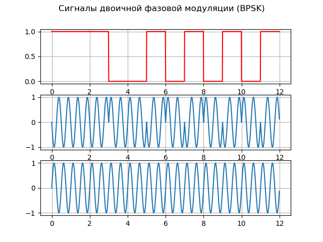
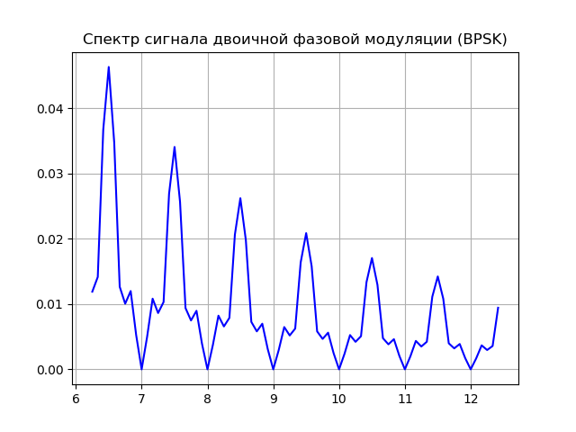
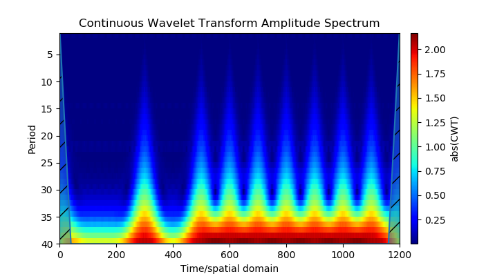
I will provide a listing explaining the basic principles of BPSK:

Listing

from scipy import* from pylab import* import numpy as np import scaleogram as scg f = 2; #f  fs = 100; #    t = arange(0,1,1/fs) #    1 / fs #      BPSK p1 = 0; p2 = pi; #     N =12#     #   bit_stream=np.random.random_integers(0, 1, N+1) #   time =[]; digital_signal =[]; PSK =[]; carrier_signal =[]; #  for ii in arange(1,N+1,1): #   if bit_stream [ii] == 0: bit = [0 for w in arange(1,len(t)+1,1)]; else: bit = [1 for w in arange(1,len(t)+1,1)]; digital_signal=hstack([digital_signal,bit ]) #  BPSK if bit_stream [ii] == 0: bit = sin (2*pi*f*t+p1); else: bit = sin (2*pi*f*t+p2); PSK=hstack([PSK,bit]) #   carrier = sin (2*f*t*pi); carrier_signal = hstack([carrier_signal,carrier]) ; time = hstack([time ,t]); t=t+1 suptitle("    (BPSK)") subplot (3,1,1); plot(time,digital_signal,'r'); grid(); subplot (3,1,2); plot (time,PSK); grid(); subplot (3,1,3); plot (time,carrier_signal); grid() show() figure() title("     (BPSK)") n = len(PSK) k = np.arange(n) T = n/fs frq = k/T frq = frq[np.arange(int(n/2))] Y = fft(PSK)/n Y = Y[range(n //2)] / max(Y[range(n // 2)]) plot(frq[75:150], abs(Y)[75:150], 'b')#    grid() #   PSK  scales = scg.periods2scales( arange(1, 40)) ax2 = scg.cws(PSK, scales=scales, figsize=(6.9,2.9)); show()

We get:

Signal source model

Navigation phase-modulated harmonic signal from a satellite or spacecraft has the form:

x = a (2 p i f_{c} t + s u m s_{n} c o s (2 p i f_{n} t)),

$x = a (2 \ pi f_ {c} t + \ sum s_ {n} cos (2 \ pi f_ {n} t)),$

where the frequency of the carrier oscillations

f_{c} = 8.4

$f_ {c} = 8.4$ Ghz.

The signal has several controlled parameters: the amplitude of the n-th modulating oscillation

s_{n},

$s_ {n},$ its frequency

f_{c}

$f_ {c}$ and the amplitude of the carrier oscillations a.

To obtain a correlation function in which its side lobes will be suppressed as much as possible and the narrowest peak of correlation will be reached, we will vary the frequencies using the values of 2, 4, 8 and 16 MHz, and the modulation index in the range from 0 to 2π with step π. I will give the program listing for such a search for the parameters of the phase-modulated function for the final result:

Listing

 # coding: utf-8 from pylab import* from scipy import signal from scipy import * T = 5e-7 #   N = 2**18 #-  delay =4 # t1 =linspace(0, T, N) t2 = linspace(0 + delay, T + delay, N) fs = (N - 1)/T #  ax = 1e-3 bx = 2e-6 ay = 2e-3 by = 3e-6 aex = 1e-3 + 30e-9 bex = 2e-6 + 10e-12 aey = 2e-3 + 30e-9 bey = 3e-6 + 10e-12 taux = ax + bx*t1 tauy = ay + by*t2 tauex = aex + bex*t1 tauey = aey + bey*t2 #  # print(" :") No1 = No2 = 0 fc = 8.4e9 #  #   A1 = 2*pi A2 = 0 A3 =2*pi A4 = 4*pi #   fm1 = 2e6 fm2 = 4e6 fm3 = 8e6 fm4 = 16e6 f = 20e6 #     ff = fc - f #   fco = 16e6 #     def korel(x,y): #  def phase_shifter1(x, t, tau, b): L = linspace(0, N, N) fexp = ifftshift((L) - ceil((N - 1)/2))/T s = ((ifft(fft(x)*exp(-1j*2*pi*tau*fexp))).real)*exp(1j*2*pi*b*fc*t) return s #   def phase_shifter2(x, t, tau, b): L = linspace(0,N,N) fexp = ifftshift((L) - ceil((N - 1)/2))/T s =((ifft(fft(x)*exp(1j*2*pi*tau*fexp))).real)*exp(-1j*2*pi*b*fc*t) return s # def heterodyning(x, t): return x*exp(-1j*2*pi*ff*t) # def filt(S): p = signal.convolve(S,h) y = p[int((n - 1)/2) : int(N+(n - 1)/2)] return y def corr(y1, y2): Y1 = fft(y1) Y2 = fft(y2) # Z = Y1*Y2.conjugate() # z = ifft(Z)/N return sqrt(z.real**2 + z.imag**2) #   def graf(c, t): c1=c[int(N/2):N] c2=c[0:int(N/2)] C = concatenate((c1, c2)) xlabel(',') ylabel('') title('   ') grid(True) plot(t*1e9 - 250, C, 'b',label="    \n    ") legend(loc='best') show() noise1 = random.uniform(-No1, No1, size = N) #   noise2 =noise1 #   x1 = heterodyning(phase_shifter1(x + noise1, t1, taux, bx), t1) y1 = heterodyning(phase_shifter1(y + noise2, t2, tauy, by), t2) n = 100001 #  #  h = signal.firwin(n, cutoff = [((f - fco) / (fs * 0.5)), ((f + fco) / (fs *0.5))], pass_zero = False) x2 = filt(x1) y2 = filt(y1) X2 = phase_shifter2(x2, t1, tauex, bex) Y2 = phase_shifter2(y2, t2, tauey, bey) Corr = corr(X2, Y2) graf(Corr, t1) #     ##for A1 in [pi/4,pi/2,pi]: ## x = cos(2*pi*fc*t1 + A1*cos(2*pi*fm1*t1)) ## y = cos(2*pi*fc*t2 + A1*cos(2*pi*fm1*t2)) ## korel(x,y) ##for fm in [ fm2,fm3,fm4]: ## A1=2*pi ## x = cos(2*pi*fc*t1 + A1*cos(2*pi*fm*t1)) ## y = cos(2*pi*fc*t2 + A1*cos(2*pi*fm*t2)) ## korel(x,y) #     ##for fm2 in [ fm1, fm2,fm3,fm4]: ## A1=2*pi ## A2=2*pi ## fm1=2e6 ## x = cos(2*pi*fc*t1 + A1*cos(2*pi*fm1*t1)+A2*np.cos(2*pi*fm2*t1)) ## y =cos(2*pi*fc*t2 + A1*cos(2*pi*fm1*t2)+A2*np.cos(2*pi*fm2*t2)) ## korel(x,y) x = cos(2*pi*fc*t1 + A1*cos(2*pi*fm1*t1)+A2*np.cos(2*pi*fm2*t1)+A3*cos(2*pi*fm3*t1)+A4*cos(2*pi*fm4*t1)) y = cos(2*pi*fc*t2 + A1*cos(2*pi*fm1*t2) +A2*cos(2*pi*fm2*t2) +A3*cos(2*pi*fm3*t2)+A4*cos(2*pi*fm4*t2)) korel(x,y)

We get:

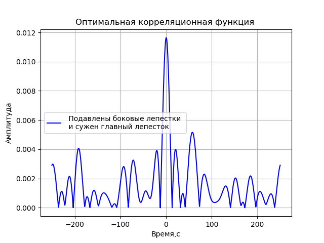
The resulting function is:

x = c o s (2 p i f_{c} t + 2 p i c o s (2 p i 10^{6} t) + 2 p i c o s (2 p i 10^{8} t) + 4 p i c o s (2 p i 10^{16} t)) . (1)

$x = cos (2 \ pi f_ {c} t + 2 \ pi cos (2 \ pi 10 ^ {6} t) +2 \ pi cos (2 \ pi 10 ^ {8} t) +4 \ pi cos (2 \ pi 10 ^ {16} t)). (1)$

Further, this function will be used to simulate VLBI.

Model of noise generator simulating interference received with the signal from space and from the atmosphere of the Earth

The function (1) of the phase-modulated navigation signal can be applied to both channels of the radio interferometer, but it should take into account the signal delay in the second channel and the noise in both channels as shown in the following listing:

Listing

 # coding: utf-8 from pylab import* from scipy import signal from scipy import * T = 5e-7 #   N = 2**16 #-  delay =1e-7 # t1 =linspace(0, T, N) t2 = linspace(0 + delay, T + delay, N) fc = 8.4e9 #  # print(" :") No1 = No2 = 0.5 noise1 = random.uniform(-No1, No1, size = N) #   noise2 =random.uniform(-No1, No1, size = N) #   x = cos(2*pi*fc*t1 + 2*pi*cos(2*pi*2*10**6*t1)+2*pi*cos(2*pi*8*10**6*t1)+4*pi*cos(2*pi*16*10**6*t1)) y = cos(2*pi*fc*t2 + 2*pi*cos(2*pi*2*10**6*t2)+2*pi*cos(2*pi*8*10**6*t2)+4*pi*cos(2*pi*16*10**6*t2)) title("    \n    ") plot(t1,x,label="  ") plot(t2,y,label="  c ") x=noise1;y=noise2 plot(t1,x,label="  ") plot(t2,y,label="  ") legend(loc='best') grid(True) figure() noise1_2 = np.random.uniform(-No1, No1, size = N) #     sko=np.std(noise1_2) mo= np.mean(noise1_2) sko=round(sko,2) mo=round(mo,2) title("  . :%s,:%s"%(sko,mo)) ylabel('   ') xlabel('  ') hist(noise1_2,bins='auto') show()

We get:

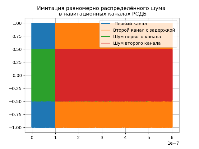
Delay delay = 1e-7 is set for demonstration, in reality it depends on the base and can reach four or more units.

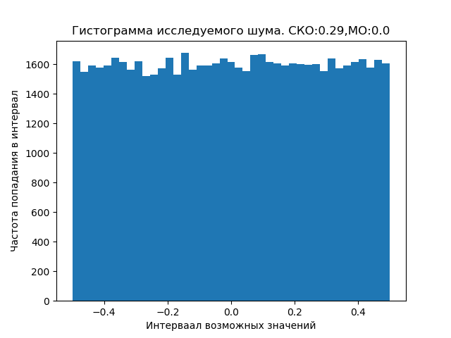
Noise, both cosmic and near-earth, can be distributed according to a law different from the uniform one, which requires special studies.

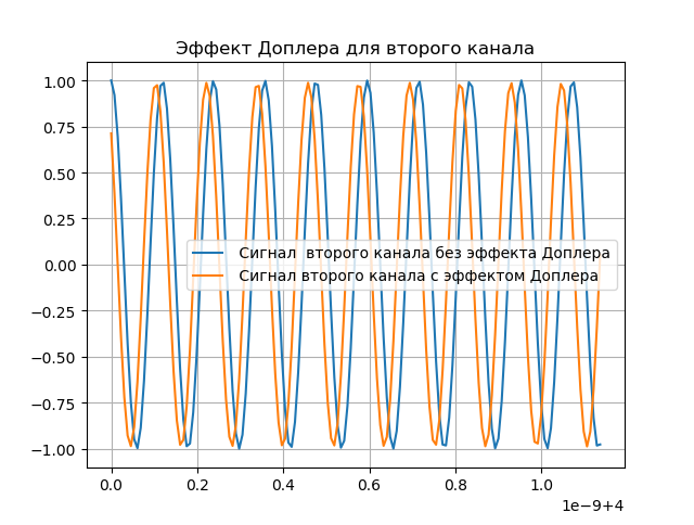
Doppler effect modeling

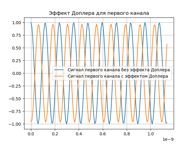
Due to the fact that the Earth has a rounded shape and rotates around its axis, the signals from space arrive at antennas with different delays. For this reason, it is required to shift the signals in time and take into account the Doppler frequency. Approximately we will assume that the delay varies according to a linear law:

t a u_{x} (t) = a_{x} + b_{x} t, (2)

$\ tau _ {x} (t) = a_ {x} + b_ {x} t, (2)$

Where

a_{x} = 1..3 c d o t 10^{- 3}

$a_ {x} = 1..3 \ cdot 10 ^ {- 3}$ ms, but

b_{x} = 1..3 c d o t 10^{- 6}

$b_ {x} = 1..3 \ cdot 10 ^ {- 6}$ ms The Doppler phase is found as a derivative of the delay:

f_{d x} = f r a c d t a u (t) d t = b_{x}, (3)

$f_ {dx} = \ frac {d \ tau (t)} {dt} = b_ {x}, (3)$

The received signal should be:

h a t x = x (t - t a u_{x}) e^{j 2 p i f_{d x} t},

$\ hat {x} = x (t- \ tau _ {x}) e ^ {j2 \ pi f_ {dx} t},$
where x (t) is the emitted signal of the spacecraft.

A demonstration of the Doppler effect is given in the following listing:

Listing

 # coding: utf-8 from pylab import* from scipy import signal from scipy import * T = 5e-7#   N = 2**16 #-  t1 =linspace(0, T, N) delay =4 # t2 = linspace(0 + delay, T + delay, N) fc = 8.4e9#  def phase_shifter1(x, t, tau, b): L = linspace(0, N, N) fexp = ifftshift((L) - ceil((N - 1)/2))/T s = ((ifft(fft(x)*exp(-1j*2*pi*tau*fexp))).real)*exp(1j*2*pi*b*fc*t) return s.real figure() title("    ") ax = 3e-3 bx = 3e-6 taux = ax + bx*t1 x = cos(2*pi*fc*t1 + 2*pi*cos(2*pi*2*10**6*t1)+2*pi*cos(2*pi*8*10**6*t1)+4*pi*cos(2*pi*16*10**6*t1)) sx=phase_shifter1(x, t1, taux, bx ) plot(t1[0:150],x[0:150],label="      ") plot(t1[0:150],sx[0:150],label="      ") grid(True) legend(loc='best') figure() title("    ") ay = 2e-3 by = 3e-6 tauy = ay + by*t2 y = cos(2*pi*fc*t2 + 2*pi*cos(2*pi*2*10**6*t2)+2*pi*cos(2*pi*8*10**6*t2)+4*pi*cos(2*pi*16*10**6*t2)) sy= phase_shifter1(y, t2, tauy, by) plot(t2[0:150],y[0:150],label="      ") plot(t2[0:150],sy[0:150],label="      ") grid(True) legend(loc='best') show()

We get:

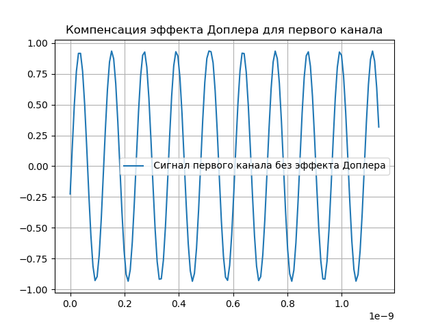
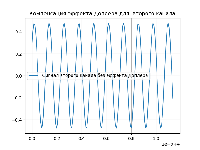
Simulation of Doppler Effect Compensation

It is obvious that the changes made to the signal should be compensated. For this purpose, there is a delay and Doppler tracking system in the system. After the signal passes through the registration system, a delay is entered:

t a u_{e x} (t) = a_{x} + b_{e x} t, (4)

$\ tau _ {ex} (t) = a_ {x} + b_ {ex} t, (4)$

It will be assumed that the delay is calculated with a certain accuracy, such that

l e f t | a_{e x} - a_{x} r i g h t | < 30

$\ left | a_ {ex} -a_ {x} \ right | <30$ ns

l e f t | b_{e x} - b_{x} r i g h t | < 10

$\ left | b_ {ex} -b_ {x} \ right | <10$ ns, i.e. it will be slightly different from the delay introduced earlier. It is clear that the delay is made with the opposite sign than the one introduced earlier.

The received signal will be:

h a t x = t i l d e x (t ​ ​ + t a u_{e x}) e^{- j 2 p i f_{d e} t} . (5)

$\ hat {x} = \ tilde {x} (t + \ tau _ {ex}) e ^ {- j2 \ pi f_ {de} t}. (5)$

Compensation of the Doppler effect is given in the following listing:

Listing

 # coding: utf-8 from pylab import* from scipy import signal from scipy import * T = 5e-7#   N = 2**16 #-  t1 =linspace(0, T, N) delay =4 # t2 = linspace(0 + delay, T + delay, N) fc = 8.4e9#  def phase_shifter1(x, t, tau, b): L = linspace(0, N, N) fexp = ifftshift((L) - ceil((N - 1)/2))/T s = ((ifft(fft(x)*exp(-1j*2*pi*tau*fexp))).real)*exp(1j*2*pi*b*fc*t) return s.real ax = 3e-3 bx = 3e-6 taux = ax + bx*t1 x = cos(2*pi*fc*t1 + 2*pi*cos(2*pi*2*10**6*t1)+2*pi*cos(2*pi*8*10**6*t1)+4*pi*cos(2*pi*16*10**6*t1)) sx=phase_shifter1(x, t1, taux, bx ) ay = 2e-3 by = 3e-6 tauy = ay + by*t2 y = cos(2*pi*fc*t2 + 2*pi*cos(2*pi*2*10**6*t2)+2*pi*cos(2*pi*8*10**6*t2)+4*pi*cos(2*pi*16*10**6*t2)) sy= phase_shifter1(y, t2, tauy, by) def phase_shifter2(x, t, tau, b): L = linspace(0,N,N) fexp = ifftshift((L) - ceil((N - 1)/2))/T s =((ifft(fft(x)*exp(1j*2*pi*tau*fexp))).real)*exp(-1j*2*pi*b*fc*t) return s.real figure() title("     ") aex = 1e-3 + 30e-9 bex = 2e-6 + 10e-12 tauex = aex + bex*t1 x1 = phase_shifter2(sx, t1, tauex, bex) plot(t1[0:150],x1[0:150],label="      ") grid(True) legend(loc='best') figure() title("     ") aey = 2e-3 + 30e-9 bey = 3e-6 + 10e-12 tauey = aey + bey*t2 y2 = phase_shifter2(sy, t2, tauey, bey) plot(t2[0:150],y2[0:150],label="      ") grid(True) legend(loc='best') show()

We get:

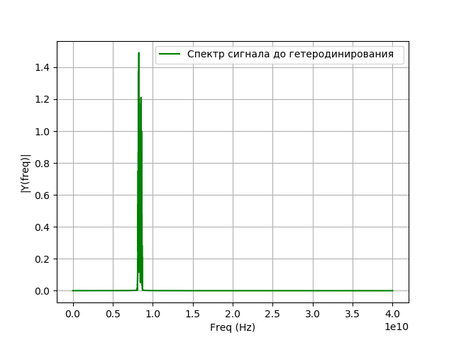
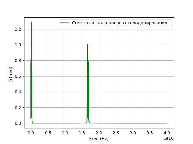
Signal heterodyning simulation

After the signal enters the recording system, a frequency conversion occurs, which is also called heterodyning. This is a non-linear transform at which from the signals of two different frequencies

f_{1}

$f_ {1}$ and

f_{2}

$f_ {2}$ difference frequency signal is released -

f = l e f t | f_{1} - f_{2} r i g h t . |

$f = \ left | f_ {1} -f_ {2} \ right. |$ The frequency of the local oscillator signal will be equal to the difference between the frequency of the signal under study and the frequency that you want to receive after the transfer. The heterodyning is performed with the help of an auxiliary generator of harmonic oscillations — a heterodyne and a nonlinear element. Mathematically, heterodyning is the multiplication of a signal by an exponent:

x_{g} = h a t x e^{j 2 p i f_{g} t}, (6)

$x_ {g} = \ hat {x} e ^ {j2 \ pi f_ {g} t}, (6)$
Where

f_{g}

$f_ {g}$ - local oscillator signal.

Program for heterodyning:

Listing

 # coding: utf-8 from pylab import* from scipy import signal from scipy import * T = 5e-7 #   N = 2**16 #-  t1 =linspace(0, T, N) fs = (N - 1)/T #  fc = 8.4e9 #  f = 20e6 #     ff = fc - f #   def spectrum_wavelet(y,a,b,c,e,st):#   n = len(y)#   k = arange(n) T = n / a frq = k / T #    frq = frq[np.arange(int(n/2))] #    Y = fft(y)/ n # FFT    Y = Y[arange(int(n/2))]/max(Y[arange(int(n/2))]) plot(frq[b:c],abs(Y)[b:c],e,label=st) #   xlabel('Freq (Hz)') ylabel('|Y(freq)|') legend(loc='best') grid(True) x = cos(2*pi*fc*t1 + 2*pi*cos(2*pi*2*10**6*t1)+2*pi*cos(2*pi*8*10**6*t1)+4*pi*cos(2*pi*16*10**6*t1)) a=fs;b=0;c=20000;e='g'; st='     ' spectrum_wavelet(x,a,b,c,e,st) show()

We get:

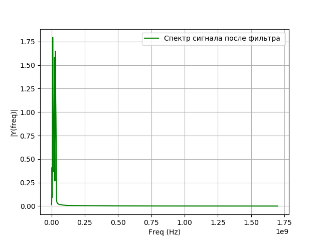
Simulation of signal filtering after heterodyning

After heterodyning, the signal goes to a bandpass filter. Bandwidth (PP) Filter

f_{p a s s} = 32

$f_ {pass} = 32$ MHz. The impulse response (IC) of the filter is calculated by the window method using the library function signal.firwin. To obtain a signal at the output of the filter, the IM filter is convolved and the signal in the time domain. The convolution integral for our case takes the form:

c h e c k x (t) = i n t_{- i n f t y}^{+ i n f t y} x_{g} (t) h (t - t^{'}) d t, (7)

$\ check {x} (t) = \ int _ {- \ infty} ^ {+ \ infty} x_ {g} (t) h (t- {t} ') dt, (7)$

where h (t) is the filter impulse response.

Convolution is found using the signal.convolve library function. Registered signal taking into account heterodyning and filtering is presented in the form of the formula

c h e c k x (t) = (h a t x (t) e^{- j 2 p i f_{g} t}) * h

$\ check {x} (t) = (\ hat {x} (t) e ^ {- j2 \ pi f_ {g} t}) * h$

where convolution is indicated by *.

Program for filtering modeling:

Listing

 # coding: utf-8 from pylab import* from scipy import signal from scipy import * T = 5e-7 #   N = 2**16 #-  t1 =linspace(0, T, N) fs = (N - 1)/T #  fc = 8.4e9 #  f = 20e6 #     ff = fc - f #   def spectrum_wavelet(y,a,b,c,e,st):#   n = len(y)#   k = arange(n) T = n / a frq = k / T #    frq = frq[np.arange(int(n/2))] #    Y = fft(y)/ n # FFT    Y = Y[arange(int(n/2))]/max(Y[arange(int(n/2))]) plot(frq[b:c],abs(Y)[b:c],e,label=st) #   xlabel('Freq (Hz)') ylabel('|Y(freq)|') legend(loc='best') grid(True) x = cos(2*pi*fc*t1 + 2*pi*cos(2*pi*2*10**6*t1)+2*pi*cos(2*pi*8*10**6*t1)+4*pi*cos(2*pi*16*10**6*t1)) def heterodyning(x, t): return x*exp(-1j*2*pi*ff*t).real z=heterodyning(x, t1) fco = 16e6 #     n = 100001 #  h = signal.firwin(n, cutoff = [((f - fco) / (fs * 0.5)), ((f + fco) / (fs *0.5))], pass_zero = False) def filt(S): p = signal.convolve(S,h) y = p[int((n - 1)/2) : int(N+(n - 1)/2)] return y q=filt(z) a=fs;b=0;c=850;e='g'; st='    ' spectrum_wavelet(q,a,b,c,e,st) show()

We get:

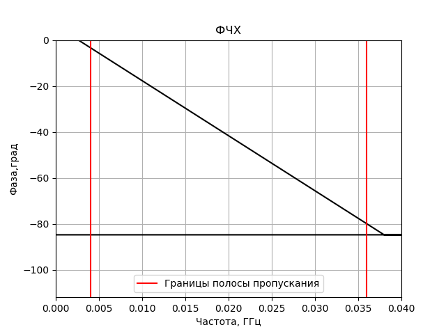
Digital signal converters for VLBI mainly use filters with finite impulse response (FIR), as they have several advantages compared to filters with infinite impulse response (IIR):

FIR filters can have a strictly linear phase response in the case of impulse response (IC) symmetry. This means that using such a filter, phase distortions can be avoided, which is especially important for radio interferometry. Filters with infinite impulse response (IIR) do not have the symmetry properties of the EM and can not have a linear phase response.
FIR filters are non-recursive, which means they are always stable. The stability of the IIR filters is not always guaranteed.
The practical implications of the fact that a limited number of bits are used to implement filters are much less significant for FIR filters.

In the above listing, the FIR bandpass filter model is implemented using the window method, the filter order was chosen such that the shape of the frequency response of the filter was close to rectangular. The number of coefficients of the simulated filter is n = 100001, that is, the order of the filter is P = 100000.

The program for building the frequency response and phase response of the received FIR filter:

Listing

 # coding: utf-8 from pylab import* from scipy import signal from scipy import * T = 5e-7 #   N = 2**16 #-  t1 =linspace(0, T, N) fs = (N - 1)/T #  fc = 8.4e9 #  f = 20e6 #     ff = fc - f #   fco = 16e6 #     n = 100001 #  h = signal.firwin(n, cutoff = [((f - fco) / (fs * 0.5)), ((f + fco) / (fs *0.5))], pass_zero = False) #  def AFC(A, n, f, deltf, min, max): plot((fftfreq (n, 1./fs)/1e9), 10*log10(abs(fft(A))), 'k') axvline((f - fco)/1e9, color = 'red', label='  ') axvline((f + fco)/1e9, color = 'red') axhline(-3, color='green', linestyle='dashdot') text(8.381, -3, repr(round(-3, 9))) xlabel(', ') ylabel(' , ') title('') grid(True) axis([(f - deltf)/1e9, (f + deltf)/1e9, min, max]) grid(True) show() #  def PFC(A, n, f, deltf, min, max): plot(fftfreq(n, 1./fs)/1e9, np.unwrap(np.angle(fft(A))), 'k') axvline((f - fco)/1e9, color='red', label='  ') axvline((f + fco)/1e9, color='red') xlabel(', ') ylabel(',') title('') axis([(f - deltf)/1e9, (f + deltf)/1e9, min, max]) #  grid(True) legend(loc='best') show() AFC(h, n, f, 20e6, -30, 1) PFC(h, n, f, 20e6, -112, 0)

We get:

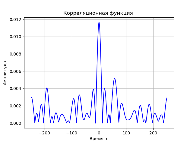
FX Correlator Model

Each signal then undergoes a Fast Fourier Transform (FFT). The FFT is implemented using the fft library function from scipy.fftpack. The resulting complex-conjugate spectra are multiplied:

S (j o m e g a) = S_{1} (j o m e g a) * S_{2} (j o m e g a) = (a_{1} + j b_{1}) * (a_{2} - j b_{2}) = a_{1} a_{2} + b_{1} b_{2} + j (b_{1} a_{2} - a_{1} b_{2})

$S (j \ omega) = S_ {1} (j \ omega) * S_ {2} (j \ omega) = (a_ {1} + jb_ {1}) * (a_ {2} -jb_ {2} ) = a_ {1} a_ {2} + b_ {1} b_ {2} + j (b_ {1} a_ {2} -a_ {1} b_ {2})$

The last action is the inverse FFT. Since the amplitude of the correlation function is of interest, the resulting signal must be converted by the formula:

A = s q r t r e^{2} + i m^{2}

$A = \ sqrt {re ^ {2} + im ^ {2}}$

Program for the correlation function without registration system distortions:

Listing

 # coding: utf-8 from pylab import* from scipy import signal from scipy import * T = 5e-7#   N = 2**16 #-  t1 =linspace(0, T, N) delay =4 # t2 = linspace(0 + delay, T + delay, N) fc = 8.4e9#  def corr(y1, y2): Y1 = fft(y1) Y2 = fft(y2) # Z = Y1*Y2.conjugate() # z = ifft(Z)/N q=sqrt(z.real**2 + z.imag**2) c1=q[int(N/2):N] c2=q[0:int(N/2)] C = concatenate((c1, c2)) xlabel(',') ylabel('') title('  ') grid(True) plot(t1*1e9 - 250, C, 'b') show() x= cos(2*pi*fc*t1 + 2*pi*cos(2*pi*2*10**6*t1)+2*pi*cos(2*pi*8*10**6*t1)+4*pi*cos(2*pi*16*10**6*t1)) y = cos(2*pi*fc*t2 + 2*pi*cos(2*pi*2*10**6*t2)+2*pi*cos(2*pi*8*10**6*t2)+4*pi*cos(2*pi*16*10**6*t2)) corr(x, y)

We get:

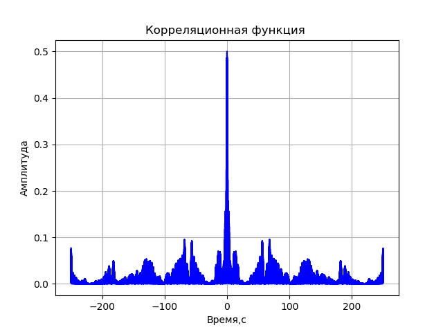
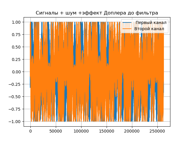
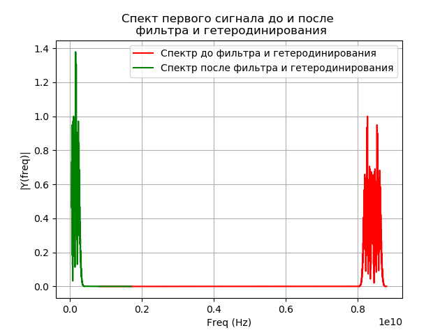
Full listing of computer model RSLB:

Listing

 # coding: utf-8 from pylab import* from scipy import signal from scipy import * T = 5e-7 #   N = 2**18 #-  delay =4 # t1 =linspace(0, T, N) t2 = linspace(0 + delay, T + delay, N) fs = (N - 1)/T #  ax = 1e-3 bx = 2e-6 ay = 2e-3 by = 3e-6 aex = 1e-3 + 30e-9 bex = 2e-6 + 10e-12 aey = 2e-3 + 30e-9 bey = 3e-6 + 10e-12 taux = ax + bx*t1 tauy = ay + by*t2 tauex = aex + bex*t1 tauey = aey + bey*t2 #  # print(" :") No1 = No2 = 0 #    # print(" :") fc = 8.4e9 #  f = 20e6 #     ff = fc - f #   fco = 16e6 #     #  def phase_shifter1(x, t, tau, b): L = linspace(0, N, N) fexp = ifftshift((L) - ceil((N - 1)/2))/T s = ((ifft(fft(x)*exp(-1j*2*pi*tau*fexp))).real)*exp(1j*2*pi*b*fc*t) return s #   def phase_shifter2(x, t, tau, b): L = linspace(0,N,N) fexp = ifftshift((L) - ceil((N - 1)/2))/T s =((ifft(fft(x)*exp(1j*2*pi*tau*fexp))).real)*exp(-1j*2*pi*b*fc*t) return s # def heterodyning(x, t): return x*exp(-1j*2*pi*ff*t) # def filt(S): p = signal.convolve(S,h) y = p[int((n - 1)/2) : int(N+(n - 1)/2)] return y def spectrum_wavelet(y,a,b,c,e,st):#   n = len(y)#   k = arange(n) T = n / a frq = k / T #    frq = frq[np.arange(int(n/2))] #    Y = fft(y)/ n # FFT    Y = Y[arange(int(n/2))]/max(Y[arange(int(n/2))]) plot(frq[b:c],abs(Y)[b:c],e,label=st) #   xlabel('Freq (Hz)') ylabel('|Y(freq)|') legend(loc='best') grid(True) def corr(y1, y2): Y1 = fft(y1) Y2 = fft(y2) # Z = Y1*Y2.conjugate() # z = ifft(Z)/N return sqrt(z.real**2 + z.imag**2) #   def graf(c, t): c1=c[int(N/2):N] c2=c[0:int(N/2)] C = concatenate((c1, c2)) xlabel(', ') ylabel('') title('  ') grid(True) plot(t*1e9 - 250, C, 'b') show() noise1 = random.uniform(-No1, No1, size = N) #   noise2 =random.uniform(-No1, No1, size = N) #   def signal_0(): x = cos(2*pi*fc*t1 + 2*pi*cos(2*pi*2*10**6*t1)+2*pi*cos(2*pi*8*10**6*t1)+4*pi*cos(2*pi*16*10**6*t1)) y = cos(2*pi*fc*t2 + 2*pi*cos(2*pi*2*10**6*t2)+2*pi*cos(2*pi*8*10**6*t2)+4*pi*cos(2*pi*16*10**6*t2)) return x,y title(" +  +   ") x,y= signal_0() x1 = heterodyning(phase_shifter1(x + noise1, t1, taux, bx), t1) plot(x1.real,label="  ") y1 = heterodyning(phase_shifter1(y + noise2, t2, tauy, by), t2) plot(y1.real,label=" ") grid(True) legend(loc='best') show() n = 100001 #  #  h = signal.firwin(n, cutoff = [((f - fco) / (fs * 0.5)), ((f + fco) / (fs *0.5))], pass_zero = False) title("- -    ") x2 = filt(x1) plot(x2.real,label="  ") y2 = filt(y1) plot(y2.real,label="  ") grid(True) legend(loc='best') show() plt.title("      \n   ") a=fs;b=400;c=4400;e='r' st="    " spectrum_wavelet(x,a,b,c,e,st) a=fs;b=20;c=850;e='g' st="    " spectrum_wavelet(x1,a,b,c,e,st) show() X2 = phase_shifter2(x2, t1, tauex, bex) Y2 = phase_shifter2(y2, t2, tauey, bey) Corr = corr(X2, Y2) graf(Corr, t1)

We get:

findings

A brief history of the development of radio astronomy is given.
Analyzed the current state of VLBI - networks.
The problems solved by means of VLBI – networks are considered.
By means of Python, a model of navigation signals with a binary (two-position) phase modulation - BPSK (binary phase shift key) is built. The model used wavelet analysis of phase modulation.
A model of signal sources is obtained, which allows one to determine modulation parameters that provide the optimal correlation function by the criterion of side lobe suppression and the maximum amplitude of the central lobe.
A model of a simplified VLBI network is obtained, which takes into account noise and the Doppler effect. Filtering features are considered using a filter with a finite impulse response.
After a brief presentation of the theory, all models are equipped with demonstration programs that allow you to track the influence of model parameters.

Source: https://habr.com/ru/post/458252/

All Articles

Mathematical model of a radio telescope with a super-long base

Introduction

Current state of VLBI - networks

Tasks solved by means of VLBI

Navigation in space by means of VLBI

Block diagram of a simplified VLBI - network

Navigation Signal Model

Signal source model

Model of noise generator simulating interference received with the signal from space and from the atmosphere of the Earth

Doppler effect modeling

Simulation of Doppler Effect Compensation

Signal heterodyning simulation

Simulation of signal filtering after heterodyning

FX Correlator Model

Full listing of computer model RSLB:

findings

More articles: