Full course in Russian can be found at this link .
The original English course is available here .

The release of new lectures is scheduled every 2-3 days.

Content

1. Interview with Sebastian Trun
2. Introduction
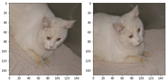
3. Cats and cats data set
4. Images of various sizes
5. Color images. Part 1
6. Color images. Part 2
7. Convolution operation on color images
8. The subsample operation on the maximum value on color images
9. CoLab: cats and dogs
10. Softmax and sigmoid
11. Check
12. Image extension
13. An exception
14. CoLab: dogs and cats. Reiteration
15. Other techniques to prevent retraining
16. Exercise: classification of color images
17. Results

Softmax and Sigmoid

In the past practical CoLab, we used the following convolutional neural network architecture:

model = tf.keras.models.Sequential([ tf.keras.layers.Conv2D(32, (3,3), activation='relu', input_shape=(150, 150, 3)), tf.keras.layers.MaxPooling2D(2, 2), tf.keras.layers.Conv2D(64, (3,3), activation='relu'), tf.keras.layers.MaxPooling2D(2,2), tf.keras.layers.Conv2D(128, (3,3), activation='relu'), tf.keras.layers.MaxPooling2D(2,2), tf.keras.layers.Conv2D(128, (3,3), activation='relu'), tf.keras.layers.MaxPooling2D(2,2), tf.keras.layers.Flatten(), tf.keras.layers.Dense(512, activation='relu'), tf.keras.layers.Dense(2, activation='softmax') ]) 

Please note that our last layer (our classifier) ​​consists of a fully connected layer with two output neurons and the softmax activation softmax :

 tf.keras.layers.Dense(2, activation='softmax') 

Another popular approach to solving binary classification problems is the use of a classifier, which consists of a fully connected layer with 1 output neuron and the sigmoid activation sigmoid :

 tf.keras.layers.Dense(1, activation='sigmoid') 

Both of these options will work well in the binary classification problem. However, it is worth bearing in mind that if you decide to use the sigmoid activation sigmoid in your classifier, you will also need to change the loss function in the model.compile() method from sparse_categorical_crossentropy to binary_crossentropy as in the example below:

 model.compile(optimizer='adam', loss='binary_crossentropy', metrics=['accuracy']) 

Validation

In previous sessions, we studied the accuracy of our convolutional neural networks using the accuracy metric on a test dataset. When we developed the convolutional neural network to classify images from the FASHION MNIST dataset, we obtained 97% accuracy on the training data set and only 92% accuracy on the test data set. All this happened because our model was retrained. In other words, our convolutional neural network began to memorize the training data set. However, we were able to learn about retraining only after we had conducted training and testing of the model on the available data by comparing the accuracy of work on the training data set and the test data set.

To avoid this problem, we often use the data set for validation:

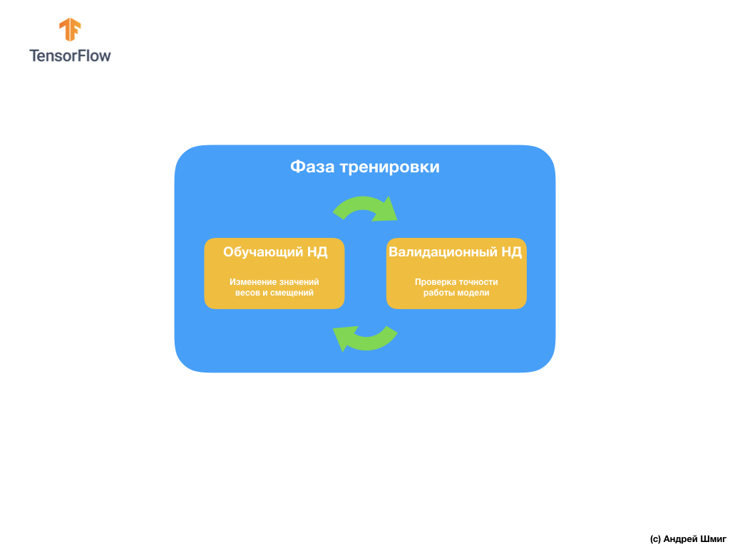
During training, our convolutional neural network "sees" only the training data set and makes decisions on how to change the values ​​of the internal parameters - weights and offsets. After each training iteration, we check the state of the model by calculating the value of the loss function on the training data set and on the validation data set. It is worth noting and paying special attention to the fact that the data from the validation set are not used anywhere by the model to adjust the values ​​of internal parameters. Checking the accuracy of the model on the validation data set only tells us how well our model is working on this very data set. Thus, the results of the model on the validation data set tell us how well our model learned how to summarize the data and apply this generalization on the new data set.

The idea is that since we do not use a validation dataset when training a model, testing the model on the validation set will allow us to understand whether the model has been retrained or not.

Let's take an example.

In CoLab, which we performed several points above, we trained our neural network for 15 iterations.

 Epoch 15/15 10/10 [===] - loss: 1.0124 - acc: 0.7170 20/20 [===] - loss: 0.0528 - acc: 0.9900 - val_loss: 1.0124 - val_acc: 0.7070 

If we look at the accuracy of the predictions on the training and validation data sets on the fifteenth training iteration, then we can see that we achieved high accuracy on the training data set and a significantly low figure on the validation data set - 0.9900 against 0.7070 .

This is an obvious sign of retraining. The neural network has memorized the training data set, therefore it works with incredible accuracy on the input data from it. However, as soon as the case shifts to checking accuracy on a validation data set that the model has not “seen”, the results are significantly reduced.

One way to avoid overtraining is to closely examine the loss function graph in the training and validation datasets throughout the training iterations:

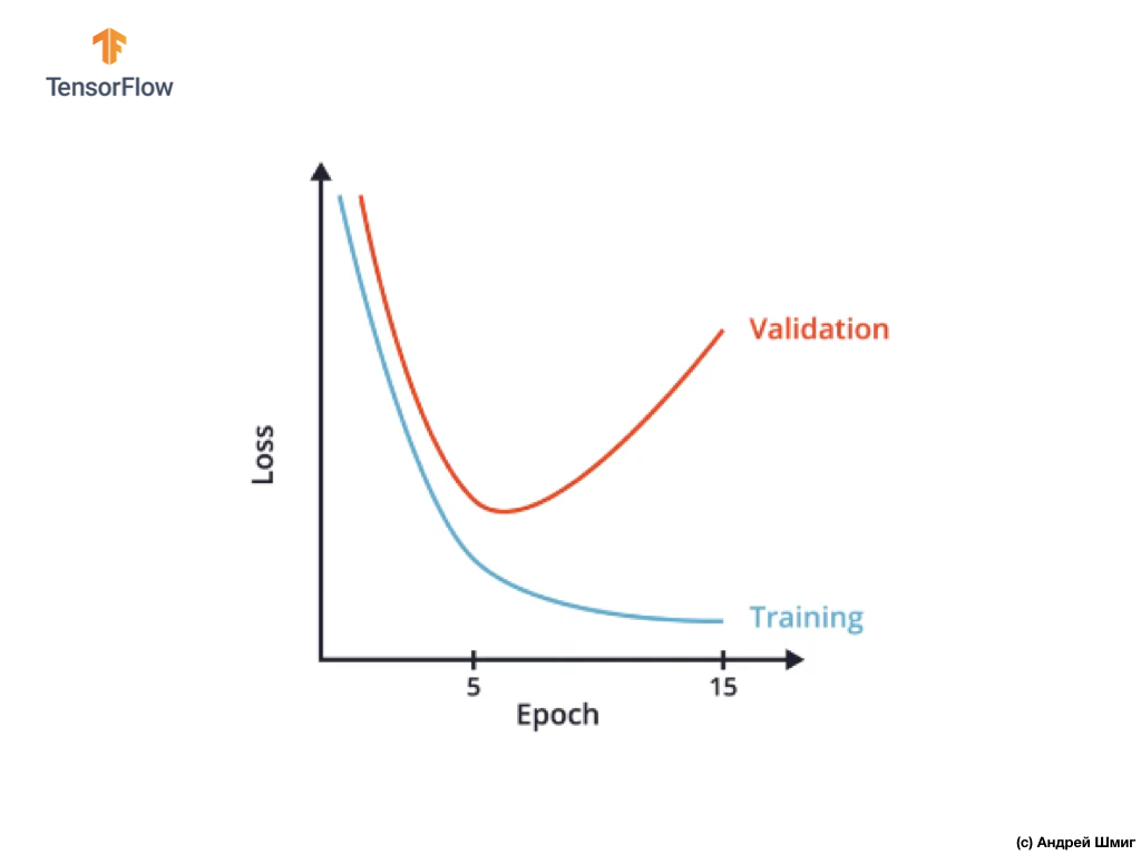
In CoLab, we built a similar graph and got something similar to the above graph of the loss function versus the training iteration.

It can be seen that after a certain training iteration, the value of the loss function on the validation data set begins to increase, while the value of the loss function on the training data set continues to decrease.

At the end of the 15th training iteration, we notice that the value of the loss function on the validation data set is extremely high, and the value of the loss function on the training data set is extremely small. Actually, this is the very indicator of the re-learning of the neural network.

Carefully looking at the graph, one can understand that literally after several training iterations, our neural network begins to simply memorize training data, which means the model's ability to generalize decreases, which leads to a deterioration in accuracy on the validation data set.

As you probably already understood, the validation data set allows us to determine the number of training iterations that need to be carried out in order for our convolutional neural network to be accurate and, at the same time, not to retrain.

Such an approach can be extremely useful if we have a choice of several architectures of convolutional neural networks:

For example, if you decide on the number of layers in a convolutional neural network, you can create several neural network architectures and then compare their accuracy using a data set for validation.

The neural network architecture, which allows you to achieve the minimum value of the loss function and will be the best to solve your problem.

The next question you might have is why create a validation data set if we already have a test data set? Can we use a test dataset for validation?

The problem is that despite the fact that we do not use the validation data set in the model training process, we use the results of the work on the test data set to improve the accuracy of the model, which means that the test data set affects the weights and displacements in the neural network.

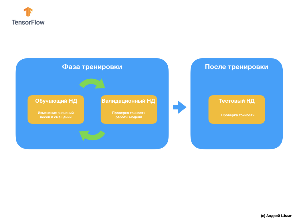
It is for this reason that we need a validation dataset, which our model has never seen before to accurately check the effectiveness of its work.

We have just figured out how a validation dataset can help us avoid retraining. In the following parts we will talk about data expansion (the so-called augmentation) and disconnections (the so-called dropout) of neurons - two popular techniques that can also help us avoid retraining.

Image extension (augmentation)

By training neural networks to define objects of a particular class, we want our neural network to find these objects regardless of their location and size in the image.

For example, imagine that we want to train our neural network to recognize dogs in images:

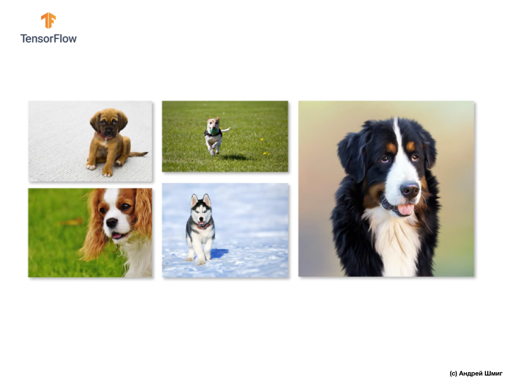
Thus, we want our neural network to determine the presence of a dog in the image, regardless of what size the dog is and in which part of the image it is, whether part of the dog is visible or the entire dog. We want to make sure that our neural network can process all these options during training.

If you are very lucky enough and you have a large set of training data, then we can safely say that you are lucky and your neural network is less likely to retrain. However, which is quite often the case, we will have to work with a limited set of images (training data), which, in turn, will lead our convolutional neural network with high probability to retrain and reduce its ability to summarize and output the desired result to data that it does not "seen" earlier.

This problem can be solved using the technique called "extension" (image augmentation). The expansion of images (data) works by creating (generating) new images for learning by applying arbitrary transformations of the original set of images from the training sample.

For example, we can take one of the original images from our training data set and apply several arbitrary transformations to it — flip it by X degrees, flip horizontally and produce an arbitrary increase.

By adding the generated images to our training data set, we thereby ensure that our neural network "sees" a sufficient number of different examples for learning. As a result of such actions, our convolutional neural network will better generalize and work on the data that it has not yet seen and we will be able to avoid retraining.

In the next section, we will learn what a dropout is — another technique for preventing model retraining.

Exception (dropout)

In this part, we will learn a new technique - a dropout, which will also help us avoid retraining the model. As we already know from the early parts, the neural network optimizes internal parameters (weights and displacements) to minimize the loss function.

One of the problems that can be encountered while learning a neural network is huge values ​​in one part of the neural network and small values ​​in another part of the neural network.

As a result, it turns out that neurons with greater weights play a greater role in the learning process, while neurons with smaller weights cease to be significant and less and less subject to change. One way to avoid this is to use an arbitrary dropout of neurons.

Dropout - the process of selectively turning off neurons in the learning process.

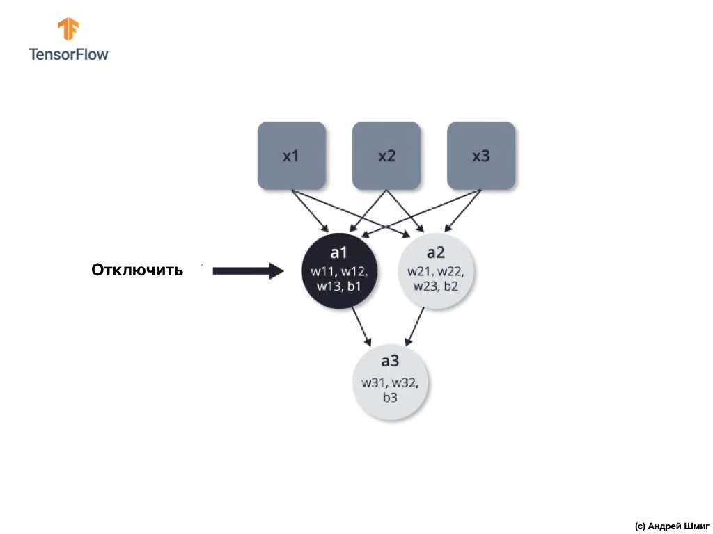
Selective disconnection of some neurons in the learning process allows active use of other neurons in learning. In the process of learning iterations, we arbitrarily disable some neurons.

Let's look at an example. Imagine that at the first training iteration we disable two black neurons highlighted in black:

The processes of direct propagation and reverse propagation occur without the use of selected two neurons.

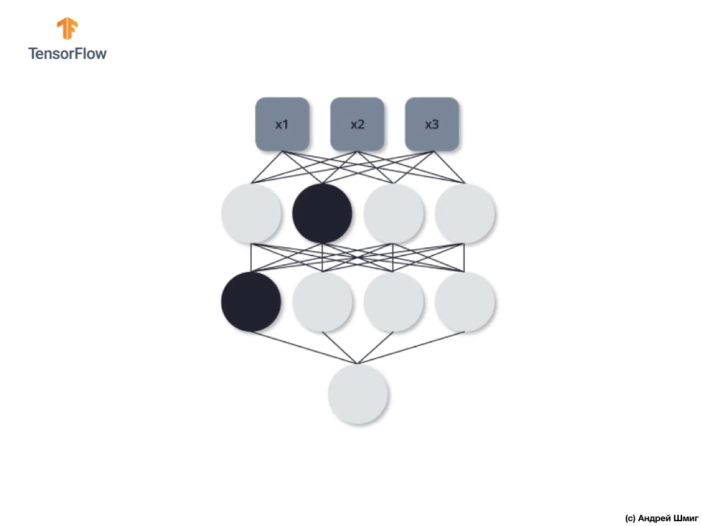
On the second training iteration, we decide not to use the following three neurons - turn them off:

As in the previous case, we do not use these three neurons in the processes of direct and reverse propagation. At the last, third learning iteration, we decide not to use these two neurons:

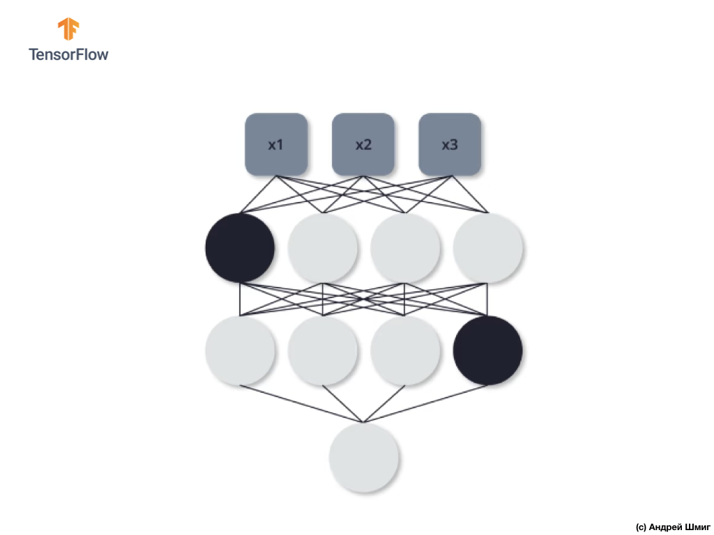
And in this case, in the processes of direct and reverse propagation, we do not use disconnected neurons. And so on.

By training our neural network so we can avoid retraining. We can say that our neural network becomes more stable, because with this approach it cannot rely absolutely on all neurons to solve the problem. Thus, other neurons begin to take a more active part in the formation of the required output value and also begin to cope with the task.

In practice, this approach requires specifying the probability of excluding each of the neurons at any learning iteration. Please note that by indicating the likelihood we may be in a situation where some neurons will shut down more often than others, and some may not be turned off at all. However, this is not a problem, because this process is performed many times and, on average, each neuron can be turned off with the same probability.

Now let's apply our theoretical knowledge in practice and refine our classifier of cats and dogs images.

CoLab: dogs and cats. Reiteration

CoLab in English is available at this link .
CoLab in Russian is available at this link .

Cats VS Dogs: classification of images with the extension

In this tutorial we will discuss how to classify images of cats and dogs. We will develop an image classifier using the tf.keras.Sequential model, and we will use tf.keras.preprocessing.image.ImageDataGenerator to load the data.

Ideas to be covered in this section:

We will gain practical experience in developing a classifier and develop an intuitive understanding of the following concepts:

1. Building a data flow model ( data input pipelines ) using the tf.keras.preprocessing.image.ImageDataGenerator class (How to effectively work with data on disk interacting with the model?)
2. Retraining - what is it and how to define it?
3. Data extension (data augmentation) and the exception method (dropout) are key techniques in the fight against retraining in pattern recognition tasks that we will implement in our model learning process.

We will follow the basic approach when developing machine learning models:

1. Explore and understand data
2. Configure Input Stream
3. Build model
4. To train a model
5. Test model
6. Improve Model / Repeat Process

Before we start ...

Before running the code in the editor, we recommend that you reset all settings in Runtime -> Reset all in the top menu. Such an action will avoid problems with low memory, if you are working in parallel or working with multiple editors.

Importing packages

Let's start by importing the right packages:

• os - reading files and directory structures;
• numpy - for some matrix operations outside TensorFlow;
• matplotlib.pyplot - plotting and displaying images from a test and validation data set.

 from __future__ import absolute_import, division, print_function, unicode_literals import os import matplotlib.pyplot as plt import numpy as np 

Import TensorFlow :

 import tensorflow as tf from tensorflow.keras.preprocessing.image import ImageDataGenerator 

 import logging logger = tf.get_logger() logger.setLevel(logging.ERROR) 

Data loading

We start the development of our classifier by loading a data set. The dataset we use is a filtered version of the Dogs vs Cats dataset from Kaggle (after all, this dataset is provided by Microsoft Research).

In the past, CoLab and I used a data set from the TensorFlow Dataset module itself, which is extremely convenient for work and testing. In this CoLab, however, we will use the tf.keras.preprocessing.image.ImageDataGenerator class to read data from disk. Therefore, we first need to download the VS Cats Dogs dataset and unzip it.

 _URL = 'https://storage.googleapis.com/mledu-datasets/cats_and_dogs_filtered.zip' zip_dir = tf.keras.utils.get_file('cats_and_dogs_filterted.zip', origin=_URL, extract=True) 

The dataset we downloaded has the following structure:

 cats_and_dogs_filtered |__ train |______ cats: [cat.0.jpg, cat.1.jpg, cat.2.jpg ...] |______ dogs: [dog.0.jpg, dog.1.jpg, dog.2.jpg ...] |__ validation |______ cats: [cat.2000.jpg, cat.2001.jpg, cat.2002.jpg ...] |______ dogs: [dog.2000.jpg, dog.2001.jpg, dog.2002.jpg ...] 

To get a full list of director you can use the following command:

 zip_dir_base = os.path.dirname(zip_dir) !find $zip_dir_base -type d -print 

Output (when starting from CoLab):

 /root/.keras/datasets /root/.keras/datasets/cats_and_dogs_filtered /root/.keras/datasets/cats_and_dogs_filtered/train /root/.keras/datasets/cats_and_dogs_filtered/train/dogs /root/.keras/datasets/cats_and_dogs_filtered/train/cats /root/.keras/datasets/cats_and_dogs_filtered/validation /root/.keras/datasets/cats_and_dogs_filtered/validation/dogs /root/.keras/datasets/cats_and_dogs_filtered/validation/cats 

Now, assign the variables the correct paths to directories with data sets for training and validation:

 base_dir = os.path.join(os.path.dirname(zip_dir), 'cats_and_dogs_filtered') train_dir = os.path.join(base_dir, 'train') validation_dir = os.path.join(base_dir, 'validation') train_cats_dir = os.path.join(train_dir, 'cats') train_dogs_dir = os.path.join(train_dir, 'dogs') validation_cats_dir = os.path.join(validation_dir, 'cats') validation_dogs_dir = os.path.join(validation_dir, 'dogs') 

We understand the data and their structure

Let's see how many images of cats and dogs we have in the test and validation data sets (directories).

 num_cats_tr = len(os.listdir(train_cats_dir)) num_dogs_tr = len(os.listdir(train_dogs_dir)) num_cats_val = len(os.listdir(validation_cats_dir)) num_dogs_val = len(os.listdir(validation_dogs_dir)) total_train = num_cats_tr + num_dogs_tr total_val = num_cats_val + num_dogs_val 

 print('    : ', num_cats_tr) print('    : ', num_dogs_tr) print('    : ', num_cats_val) print('    : ', num_dogs_val) print('--') print('     : ', total_train) print('     : ', total_val) 

Conclusion:

     : 1000     : 1000     : 500     : 500 --      : 2000      : 1000 

Setting Model Parameters

For convenience, we will make setting variables that we need for further data processing and model training, in a separate declaration:

 BATCH_SIZE = 100 #          IMG_SHAPE = 150 #        

Data extension

Re-training usually occurs when there are few training examples in our data set. One of the ways to eliminate the lack of data is to expand them to the required number of instances and the desired variability. Data expansion is the process of generating data from existing instances by applying various transformations to the original data set. The goal of this method is to increase the number of unique input instances that the model will never see again, which, in turn, will allow the model to better generalize the input data and show greater accuracy on the validation data set.

Using tf.keras we can implement similar random transformations and the generation of new images through the ImageDataGenerator class. It will be enough for us to pass in the form of parameters various transformations that we would like to apply to the images, while the class itself will take care of the rest during the training of the model.

To begin, let's write a function that will display images obtained as a result of random transformations. Then we take a closer look at the transformations used in the process of expanding the original data set.

 def plotImages(images_arr): fig, axes = plt.subplots(1, 5, figsize=(20,20)) axes = axes.flatten() for img, ax in zip(images_arr, axes): ax.imshow(img) plt.tight_layout() plt.show() 

Horizontal flip

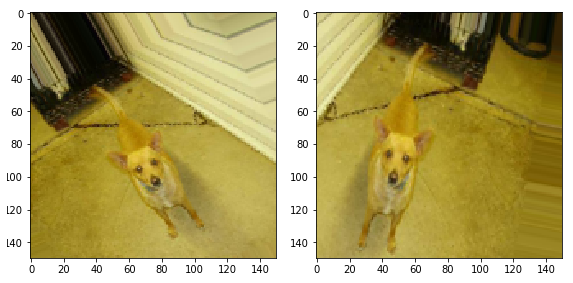
We can start with a simple transformation - horizontal image flipping. Let's see how this transformation will look applied to our source images. To achieve such a transformation, you must pass the parameter horizontal_flip=True constructor of the ImageDataGenerator class.

 image_gen = ImageDataGenerator(rescale=1./255, horizontal_flip=True) train_data_gen = image_gen.flow_from_directory(batch_size=BATCH_SIZE, directory=train_dir, shuffle=True, target_size=(IMG_SHAPE, IMG_SHAPE)) 

Conclusion:

 Found 2000 images belonging to 2 classes. 

. ( ) .

 augmented_images = [train_data_gen[0][0][0] for i in range(5)] plotImages(augmented_images) 

(2 5 ):

. 45.

 image_gen = ImageDataGenerator(rescale=1./255, rotation_range=45) train_data_gen = image_gen.flow_from_directory(batch_size=BATCH_SIZE, directory=train_dir, shuffle=True, target_size=(IMG_SHAPE, IMG_SHAPE)) 

Conclusion:

 Found 2000 images belonging to 2 classes. 

— 5 . ( ) .

 augmented_images = [train_data_gen[0][0][0] for i in range(5)] plotImages(augmented_images) 

(2 5):

— 50%.

 image_gen = ImageDataGenerator(rescale=1./255, zoom_range=0.5) train_data_gen = image_gen.flow_from_directory(batch_size=BATCH_SIZE, directory=train_dir, shuffle=True, target_size=(IMG_SHAPE, IMG_SHAPE)) 

Conclusion:

 Found 2000 images belonging to 2 classes. 

, — 5 . ( ) .

 augmented_images = [train_data_gen[0][0][0] for i in range(5)] plotImages(augmented_images) 

(2 5 ):

, , , ImageDataGenerator .

— , 45 , , , .

 image_gen_train = ImageDataGenerator( rescale=1./255, rotation_range=40, width_shift_range=0.2, height_shift_range=0.2, shear_range=0.2, zoom_range=0.2, horizontal_flip=True, fill_mode='nearest' ) train_data_gen = image_gen_train.flow_from_directory(batch_size=BATCH_SIZE, directory=train_dir, shuffle=True, target_size=(IMG_SHAPE, IMG_SHAPE), class_mode='binary') 

Conclusion:

 Found 2000 images belonging to 2 classes. 

, .

 augmented_images = [train_data_gen[0][0][0] for i in range(5)] plotImages(augmented_images) 

(2 5):

, , , . , , .

 image_gen_val = ImageDataGenerator(rescale=1./255) val_data_gen = image_gen_val.flow_from_directory(batch_size=BATCH_SIZE, directory=validation_dir, target_size=(IMG_SHAPE, IMG_SHAPE), class_mode='binary') 

4 .

0.5. , 50% 0. .

512 relu . — — softmax .

 model = tf.keras.models.Sequential([ tf.keras.layers.Conv2D(32, (3,3), activation='relu', input_shape=(IMG_SHAPE, IMG_SHAPE, 3)), tf.keras.layers.MaxPooling2D(2, 2), tf.keras.layers.Conv2D(64, (3, 3), activation='relu'), tf.keras.layers.MaxPooling2D(2, 2), tf.keras.layers.Conv2D(128, (3, 3), activation='relu'), tf.keras.layers.MaxPooling2D(2, 2), tf.keras.layers.Conv2D(128, (3, 3), activation='relu'), tf.keras.layers.MaxPooling2D(2, 2), tf.keras.layers.Dropout(0.5), tf.keras.layers.Flatten(), tf.keras.layers.Dense(512, activation='relu'), tf.keras.layers.Dense(2, activation='softmax') ]) 

adam . sparse_categorical_crossentropy . , accuracy metrics :

 model.compile(optimizer='adam', loss='sparse_categorical_crossentropy', metrics=['accuracy']) 

summary :

 model.summary() 

Conclusion:

 Model: "sequential" _________________________________________________________________ Layer (type) Output Shape Param # ================================================================= conv2d (Conv2D) (None, 148, 148, 32) 896 _________________________________________________________________ max_pooling2d (MaxPooling2D) (None, 74, 74, 32) 0 _________________________________________________________________ conv2d_1 (Conv2D) (None, 72, 72, 64) 18496 _________________________________________________________________ max_pooling2d_1 (MaxPooling2 (None, 36, 36, 64) 0 _________________________________________________________________ conv2d_2 (Conv2D) (None, 34, 34, 128) 73856 _________________________________________________________________ max_pooling2d_2 (MaxPooling2 (None, 17, 17, 128) 0 _________________________________________________________________ conv2d_3 (Conv2D) (None, 15, 15, 128) 147584 _________________________________________________________________ max_pooling2d_3 (MaxPooling2 (None, 7, 7, 128) 0 _________________________________________________________________ dropout (Dropout) (None, 7, 7, 128) 0 _________________________________________________________________ flatten (Flatten) (None, 6272) 0 _________________________________________________________________ dense (Dense) (None, 512) 3211776 _________________________________________________________________ dense_1 (Dense) (None, 2) 1026 ================================================================= Total params: 3,453,634 Trainable params: 3,453,634 Non-trainable params: 0 _________________________________________________________________ 

!

( ImageDataGenerator ) fit_generator fit :

 EPOCHS = 100 history = model.fit_generator( train_data_gen, steps_per_epoch=int(np.ceil(total_train / float(BATCH_SIZE))), epochs=EPOCHS, validation_data=val_data_gen, validation_steps=int(np.ceil(total_val / float(BATCH_SIZE))) ) 

:

 acc = history.history['acc'] val_acc = history.history['val_acc'] loss = history.history['loss'] val_loss = history.history['val_loss'] epochs_range = range(EPOCHS) plt.figure(figsize=(8,8)) plt.subplot(1, 2, 1) plt.plot(epochs_range, acc, label='  ') plt.plot(epochs_range, val_acc, label='  ') plt.legend(loc='lower right') plt.title('     ') plt.subplot(1, 2, 2) plt.plot(epochs_range, loss, label='  ') plt.plot(epochs_range, val_loss, label='  ') plt.legend(loc='upper right') plt.title('     ') plt.savefig('./foo.png') plt.show() 

Conclusion:

, :

1. : ( ).
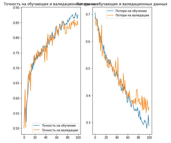
2. (.. augmentation) : .
3. / (.. dropout) : ( , ).

, . .

:

CoLab .
CoLab .

. CoLab . CoLab . CoLab , .

CoLab. CoLab , , .

Enjoy!

# tf.keras

CoLab . tf.keras.Sequential , ImageDataGenerator .

. os , numpy python- numpy- , , matplotlib.pyplot .

 from __future__ import absolute_import, division, print_function, unicode_literals import os import numpy as np import glob import shutil import matplotlib.pyplot as plt 

TODO: TensorFlow Keras-

TensorFlow tf Keras- , . , ImageDataGenerator - Keras .

 #   

Data loading

— . .

.

 _URL = "https://storage.googleapis.com/download.tensorflow.org/example_images/flower_photos.tgz" zip_file = tf.keras.utils.get_file(origin=_URL, fname="flower_photos.tgz", extract=True) base_dir = os.path.join(os.path.dirname(zip_file), 'flower_photos') 

, , 5 :

1. Roses
3. Dandelions
4. Sunflowers
5. Tulips

:

 classes = ['', '', '', '', ''] 

, , :

 flower_photos |__ diasy |__ dandelion |__ roses |__ sunflowers |__ tulips 

. . , .

2 train val 5 - ( ). , 80% , 20% . :

 flower_photos |__ diasy |__ dandelion |__ roses |__ sunflowers |__ tulips |__ train |______ daisy: [1.jpg, 2.jpg, 3.jpg ....] |______ dandelion: [1.jpg, 2.jpg, 3.jpg ....] |______ roses: [1.jpg, 2.jpg, 3.jpg ....] |______ sunflowers: [1.jpg, 2.jpg, 3.jpg ....] |______ tulips: [1.jpg, 2.jpg, 3.jpg ....] |__ val |______ daisy: [507.jpg, 508.jpg, 509.jpg ....] |______ dandelion: [719.jpg, 720.jpg, 721.jpg ....] |______ roses: [514.jpg, 515.jpg, 516.jpg ....] |______ sunflowers: [560.jpg, 561.jpg, 562.jpg .....] |______ tulips: [640.jpg, 641.jpg, 642.jpg ....] 

, , . .

 for cl in classes: img_path = os.path.join(base_dir, cl) images = glob.glob(img_path + '/*.jpg') print("{}: {} ".format(cl, len(images))) train, val = images[:round(len(images)*0.8)], images[round(len(images)*0.8):] for t in train: if not os.path.exists(os.path.join(base_dir, 'train', cl)): os.makedirs(os.path.join(base_dir, 'train', cl)) shutil.move(t, os.path.join(base_dir, 'train', cl)) for v in val: if not os.path.exists(os.path.join(base_dir, 'val', cl)): os.makedirs(os.path.join(base_dir, 'val', cl)) shutil.move(v, os.path.join(base_dir, 'val', cl)) 

:

 train_dir = os.path.join(base_dir, 'train') val_dir = os.path.join(base_dir, 'val') 

, , , . — (.. augmentation) . . , , — , . .

tf.keras , — ImageDataGenerator . .

. — () batch_size , IMG_SHAPE .

TODO:

100 batch_size 150 IMG_SHAPE :

 batch_size = IMG_SHAPE = 

TODO:

ImageDataGenerator , , . .flow_from_directory . , , , .

 image_gen = train_data_gen = 

5 :

 def plotImages(images_arr): fig, axes = plt.subplots(1, 5, figsize=(20,20)) axes = axes.flatten() for img, ax in zip(images_arr, axes): ax.imshow(img) plt.tight_layout() plt.show() augmented_images = [train_data_gen[0][0][0] for i in range(5)] plotImages(augmented_images) 

TODO:

, ImageDataGenerator 45 . .flow_from_directory . , , , .

 image_gen = train_data_gen = 

5 :

 augmented_images = [train_data_gen[0][0][0] for i in range(5)] plotImages(augmented_images) 

TODO:

, ImageDataGenerator 50%. .flow_from_directory . , , , .

 image_gen = train_data_gen = 

5 :

 augmented_images = [train_data_gen[0][0][0] for i in range(5)] plotImages(augmented_images) 

TODO:

, ImageDataGenerator :

• 45
• 50%
• 0.15
• 0.15

flow_from_directory . , , , .

 image_gen_train = train_data_gen = 

5 :

 augmented_images = [train_data_gen[0][0][0] for i in range(5)] plotImages(augmented_images) 

TODO:

. , , ImageDataGenerator , . flow_from_directory . , , . .

 image_gen_val = val_data_gen = 

TODO:

, 3 — . 16 , — 32 , — 64 . 33. 22.

Flatten , 512 . 5 , softmax . relu . , , 20%.

 model = 

TODO:

, adam sparse_categorical_crossentropy . , compile(...) .

 #   

TODO:

, fit_generator fit , . fit_generator ImageDataGenerator . 80 , fit_generator -.

 epochs = history = 

TODO: /

, :

 acc = val_acc = loss = val_loss = epochs_range = 

TODO:

( + ) 512 . . . , , .. , ImageDataGenerator — . , .

?

Results

.

RGB- :

• : , ( );
• : 3D-;
• RGB- : 3 : , ;
• : (). , (). — .
• : . , .
• : . , .

:

• : , .
• : .
• () : .

. , . .

… call-to-action — , share :)
YouTube
Telegram
In contact with