Neural networks and deep learning: online tutorial, chapter 1

Note

Before you is a translation of the free online book by Michael Nielsen "Neural Networks and Deep Learning", distributed under the Creative Commons Attribution-NonCommercial 3.0 Unported License . The motivation for its creation was the successful experience of translating a textbook on programming, " Expressive JavaScript ." The book on neural networks is also quite popular, the authors of English-language articles actively refer to it. I did not find her translations, except for the translation of the beginning of the first chapter with abbreviations .

Those who want to thank the author of the book can do it on its official page , transfer via PayPal or Bitcoin. For support of the translator on Habré there is a form "to support the author".

Introduction

This tutorial will tell you in detail about such concepts as:
')

• Neural networks are an excellent program paradigm created under the influence of biology, which allows computers to learn from observations.
• Deep learning is a powerful set of neural network training techniques.

Neural networks (NN) and deep learning (GO) today provide the best solution to many problems from the areas of image recognition, voice and natural language processing. This tutorial will teach you many of the key concepts underlying NA and GO.

What is this book about

The National Assembly is one of the most beautiful programming paradigms ever invented by man. With the standard programming approach, we tell the computer what to do, we break up large tasks into many small ones, we precisely define tasks that the computer will easily perform. In the case of the National Assembly, on the contrary, we do not tell the computer how to solve the problem. He learns this himself on the basis of “observations” of the data, “inventing” his own solution of the task.

Automated data-based learning sounds promising. However, until 2006, we did not know how to train NAs so that they could outperform the more traditional approaches, with the exception of a few special cases. In 2006, teaching techniques of the so-called deep neural networks (GNS). Now these techniques are known as deep learning (GO). They continued to be developed, and today the STS and civil defense have achieved amazing results in many important tasks related to computer vision, speech recognition and natural language processing. On a large scale, companies such as Google, Microsoft and Facebook are deploying them.

The purpose of this book is to help you master the key concepts of neural networks, including modern GO techniques. Having worked with the textbook, you will write a code that uses NA and GO to solve complex problems of recognition of patterns. You will have a foundation for the use of the National Assembly and Civil Defense in the approach to solving your own problems.

Principle-based approach

One of the beliefs underlying the book is that it is better to master a firm understanding of the key principles of the National Assembly and civil society than to grab knowledge from a long list of different ideas. If you understand key ideas well, you will quickly understand other new material. In the programmer's language, we can say that we will study the basic syntax, libraries, and data structures of the new language. You may recognize only a small fraction of the entire language — many languages ​​have vast standard libraries — but you can understand new libraries and data structures quickly and easily.

So, this book is categorically not a teaching material on how to use any particular library for the National Assembly. If you just want to learn how to work with the library - do not read the book! Find the library you need, and work with training materials and documentation. But keep in mind: although this approach has an advantage in instant problem solving, if you want to understand exactly what is happening inside the National Assembly, if you want to master ideas that will be relevant even after many years, then it will not be enough for you just to study some fashionable library. You need to understand the reliable and long-term ideas underlying the work of the National Assembly. Technology comes and goes, but ideas are forever.

Practical approach

We will learn the basic principles on the example of a specific task: learning computer to recognize handwritten numbers. Using traditional approaches to programming, this task is extremely difficult to solve. However, we can solve it quite well with a simple NA and a few dozen lines of code, without any special libraries. Moreover, we will gradually improve this program, consistently incorporating into it more and more key ideas about the National Assembly and Civil Defense.

Such a practical approach means that you will need some programming experience. But you don't have to be a professional programmer. I wrote python code (version 2.7), which should be understandable, even if you did not write python programs. In the process of studying, we will create our own library for the National Assembly, which you can use for experiments and further training. All code can be downloaded by reference . Having finished the book, or in the process of reading, you can choose one of the more complete libraries for the National Assembly, adapted for use in real projects.

The mathematical requirements for understanding the material are rather average. Most chapters have mathematical parts, but usually they are elementary algebra and graphs of functions. Sometimes I use more advanced mathematics, but I structured the material so that you can understand it, even if some details will elude you. Most of all, mathematics is used in Chapter 2, where a bit of mathematical analysis and linear algebra are required. For those to whom they are not familiar, I begin chapter 2 with an introduction to mathematics. If it seems complicated to you, just skip the chapter down to the debriefing. In any case, do not worry about it.

The book is rarely both oriented towards an understanding of principles and a practical approach. But I think it is better to study on the basis of the fundamental ideas of the National Assembly. We will write working code, and not just study abstract theory, and this code you can explore and expand. In this way, you will understand the basics, both theory and practice, and will be able to study further.

Exercises and tasks

The authors of technical books often warn the reader that he just needs to perform all the exercises and solve all the problems. When reading such warnings to me, they always seem a bit strange. Does anything bad happen to me if I do not do the exercises and solve the problems? Of course not. I will simply save time due to less deep understanding. Sometimes it's worth it. Sometimes not.

What should be done with this book? I advise you to try to do most of the exercises, but do not try to solve most of the tasks.

You need to do most of the exercises because these are basic checks for understanding the material correctly. If you can't do the exercise with relative ease, you probably missed something fundamental. Of course, if you really get stuck on an exercise - drop it, maybe it's some slight misunderstanding, or maybe I haven't formulated anything well. But if most exercises cause you trouble, then you most likely need to reread the previous material.

Tasks are another matter. They are more difficult exercises, and with some you have to hard. It is annoying, but, of course, patience in the face of such disappointment is the only way to truly understand and assimilate the subject.

So I do not recommend solving all problems. Even better - pick your own project. Maybe you want to use the NA to classify your music collection. Or to predict the value of shares. Or something else. But find an interesting project for you. And then you can ignore the tasks from the book, or use them purely as inspiration for working on your project. Problems with your own project will teach you more than working with any number of tasks. Emotional involvement is a key factor in mastery.

Of course, while you may not have such a project. This is normal. Solve problems for which you feel internal motivation. Use material from the book to help yourself in finding ideas for personal creative projects.

Chapter 1

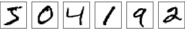
The human visual system is one of the wonders of the world. Consider the following sequence of handwritten numbers:



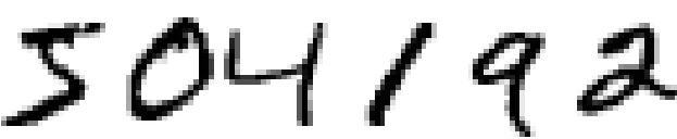
Most people read them easily, like 504192. But this simplicity is deceptive. In each hemisphere of the brain, a person has a primary visual cortex , also known as V1, which contains 140 million neurons and tens of billions of connections between them. At the same time, not only V1, but a whole sequence of brain regions - V2, V3, V4 and V5 - are involved in the increasingly complex image processing. We carry a supercomputer in our head, tuned by evolution for hundreds of millions of years, and perfectly adapted for understanding the visible world. Recognizing handwritten numbers is not easy. It’s just that we, people, are amazingly, surprisingly well aware of what our eyes show us. But almost all this work is done unconsciously. And usually we don’t attach importance to the complexity of our visual systems.

The difficulty of recognizing visual patterns becomes apparent when you try to write a computer program to recognize such figures as those given above. What seems easy in our performance suddenly turns out to be extremely difficult. A simple concept of how we recognize forms - “the nine at the top has a loop, and the vertical dash at the bottom right” - is not so simple for an algorithmic expression. Trying to formulate these rules clearly, you quickly get stuck in the quagmire of exceptions, pitfalls and special cases. The task seems hopeless.

NA approach to solving the problem differently. The idea is to take a variety of handwritten numbers, known as teaching examples,



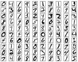
and develop a system capable of learning from these examples. In other words, NA uses examples to automatically build rules for the recognition of handwritten numbers. Moreover, by increasing the number of training examples, the network can learn more about handwritten numbers and improve its accuracy. So, although I have given above 100 training examples, we may be able to create a better handwritten recognizer using thousands or even millions and billions of teaching examples.

In this chapter, we will write a computer program that implements the NA, learning to recognize handwritten numbers. The program will be only 74 lines long, and will not use special libraries for NA. However, this short program will be able to recognize handwritten numbers with an accuracy of more than 96%, without requiring human intervention. Moreover, in later chapters we will develop ideas that can improve accuracy up to 99% or more. In fact, the best commercial NAs do the job so well that they are used by banks to process checks, and the postal service does it to recognize addresses.

We concentrate on handwriting recognition, since this is a great prototype of a task for studying NA. Such a prototype is ideal for us: it is a difficult task (recognizing handwritten numbers is not an easy task), but not so difficult that it requires an extremely complex solution or vast computational power. Moreover, it is a great way to develop more complex techniques such as GO. Therefore, in the book we will constantly return to the problem of handwriting recognition. Later we will discuss how these ideas can be applied to other tasks of computer vision, speech recognition, processing of natural language and other areas.

Of course, if the purpose of this chapter was only to write a handwritten number recognition program, the chapter would be much shorter! However, in the process, we will develop many key ideas related to NA, including two important types of artificial neuron ( perceptron and sigmoid neuron), and the standard NA learning algorithm, stochastic gradient descent . In the text, I concentrate on explaining why everything is done that way, and on shaping your understanding of the National Assembly. This requires a longer conversation than if I simply presented the basic mechanics of what is happening, but it is worth a deeper understanding that you will have. Among other advantages - by the end of the chapter you will understand what GO is and why it is so important.

Perceptrons

What is a neural network? To begin, I will talk about one type of artificial neuron, which is called the perceptron. Perceptrons came up with the scientist Frank Rosenblatt in the 1950s and 1960s, inspired by the early work of Warren McCulloch and Walter Pitts . Today, other models of artificial neurons are used more often - in this book, and most modern works on NA, they mostly use the sigmoid model of the neuron. We will meet her soon. But to understand why sigmoid neurons are defined this way, it is worth spending time analyzing the perceptron.

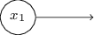
So how do perceptrons work? The perceptron accepts several binary numbers x ₁ , x ₂ , ... as an input and produces one binary number:



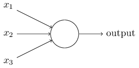
In this example, the perceptron has three input numbers, x ₁ , x ₂ , x ₃ . In general, there may be more or less. Rosenblatt proposed a simple rule for calculating the result. He introduced weights, w ₁ , w ₂ , real numbers expressing the importance of the corresponding input numbers for the results. The output of a neuron, 0 or 1, is determined by whether the weighted sum is less than or greater than a certain [threshold] threshold. $$$\ sum_j w_jx_j$ . Like weights, the threshold is a real number, a parameter of a neuron. In mathematical terms:

$$

$$output = \ begin {cases} 0 ~ if ~ \ sum_j w_jx_j \ leq threshold \\ 1 ~ if ~ \ sum_j w_jx_j> threshold \ end {cases} \ tag {1}$$

That's all the description of the work of the perceptron!

Such is the basic mathematical model. A perceptron can be thought of as a decision-making device, weighing evidence. Let me give you a not very realistic, but a simple example. Let's say the weekend is coming, and you have heard that a cheese festival will be held in your city. You like cheese, and you try to decide whether to go to the festival or not. You can decide by weighing three factors:

1. Is the weather good?
2. Does your partner want to go with you?
3. Is the festival far from the public transport stop? (You do not have a car).

These three factors can be represented by binary variables x ₁ , x ₂ , x ₃ . For example, x ₁ = 1 if the weather is good and 0 if it is bad. x ₂ = 1 if your partner wants to go, and 0 if not. Same for x ₃ .

Now, let's say you are a fan of cheese so much that you are ready to go to the festival, even if your partner is not interested, and it is difficult to get to him. But maybe you just hate bad weather, and in the event of bad weather, you will not go to the festival. You can use perceptrons to model such a decision making process. One way is to choose the weight w ₁ = 6 for the weather, and w ₂ = 2, w ₃ = 2 for other conditions. A higher w ₁ value means that the weather matters to you much more than whether your partner joins you, or whether the festival is close to a halt. Finally, let's say you choose a threshold for the perceptron 5. With these options, the perceptron implements the desired decision-making model, returning 1 when the weather is bad and 0 when it is bad. The partner’s wish and the proximity of the stop do not affect the output value.

By changing weights and thresholds, we can get different decision making models. For example, let's say take threshold 3. Then the perceptron decides that you need to go to the festival, either when the weather is fine, or when the festival is near the stop and your partner agrees to go with you. In other words, the model is different. Lowering the threshold means more you want to go to the festival.

Obviously, the perceptron is not a complete human decision-making model! But this example shows how a perceptron can weigh different types of evidence to make decisions. It seems possible that a complex network of perceptrons can make very complex decisions:



In this network, the first column of perceptrons — what we call the first layer of perceptrons — makes three very simple decisions, weighing the input evidence. What about perceptrons from the second layer? Each of them makes a decision, weighing the results of the first decision layer. In this way, the perceptron of the second layer can make a decision on a more complex and abstract level, compared to the perceptron of the first layer. And even more complex decisions can be made by perceptrons on the third layer. In this way, a multilayer network of perceptrons can be involved in making complex decisions.

By the way, when I determined the perceptron, I said that it has only one output value. But in the network at the top, the perceptrons look like they have several output values. In fact, they have only one way out. The set of output arrows is simply a convenient way to show that the output of the perceptron is used as the input of several other perceptrons. This is less cumbersome than drawing one forked exit.

Let's simplify the description of perceptrons. Condition $$$\ sum_j w_jx_j> treshold$ awkward, and we can agree on two changes to the record to simplify it. The first is to record $$$\ sum_j w_jx_j$ as a dot product, $$$w \ cdot x = \ sum_j w_jx_j$ , where w and x are vectors whose components are weights and input data, respectively. The second is to transfer the threshold to another part of the inequality, and replace it with a value known as the perceptron offset [bias], $$$b \ equiv −threshold$ . Using offset instead of threshold, we can rewrite the perceptron rule:

$$

$$output = \ begin {cases} 0 ~ if ~ w \ cdot x + b \ leq 0 \\ 1 ~ if ~ w \ cdot x + b> 0 \ end {cases} \ tag {2}$$

The offset can be represented as a measure of how easy it is to obtain the value 1 at the output from the perceptron. Or, in biological terms, displacement is a measure of how easy it is to make the perceptron activate. It is extremely easy to give out a perceptron with a very large offset 1. But with a very large negative offset, this is difficult to do. Obviously, the introduction of an offset is a small change in the description of perceptrons, but later we will see that it leads to a further simplification of the record. Therefore, below we will not use the threshold, but will always use the offset.

I described the perceptrons in terms of the method of weighing evidence with a view to making a decision. Another way to use them is to compute elementary logical functions, which we usually consider basic computations, such as AND, OR, and NAND. Suppose, for example, that we have a perceptron with two inputs, the weight of each of which is -2, and its offset is 3. Here it is:



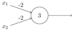
Input data 00 gives output 1, because (−2) ∗ 0 + (- 2) ∗ 0 + 3 = 3 is greater than zero. The same calculations say that input data 01 and 10 give 1. But 11 at the input gives 0 at the output, because (−2) ∗ 1 + (- 2) ∗ 1 + 3 = −1, less than zero. Therefore, our perceptron implements the NAND function!

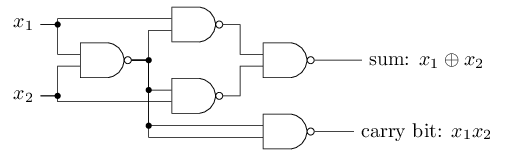
This example shows that you can use perceptrons to compute basic logic functions. In fact, we can use networks of perceptrons to calculate any logical functions at all. The fact is that the logical NAND gate is universal for computing — any calculation can be built on its basis. For example, you can use NAND gates to create a contour that folds two bits, x ₁ and x ₂ . To do this, calculate the bitwise sum. $$$x_1 \ oplus x_2$ and the carry flag , which is 1 when both x ₁ and x ₂ are 1 - that is, the carry flag is simply the result of a bitwise multiplication x ₁ x ₂ :



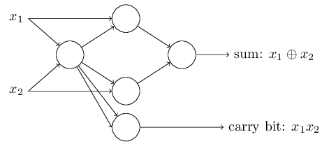
To get an equivalent network of perceptrons, we replace all NAND gates with two inputs, each with a weight of -2, and with an offset of 3. This is the resulting network. Note that I moved the perceptron corresponding to the right bottom valve, just to make it easier to draw arrows:



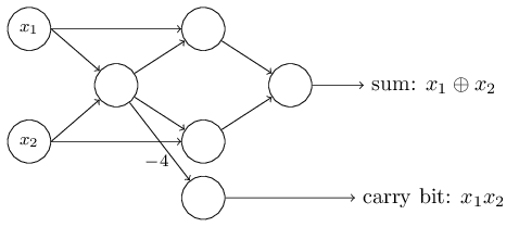
One notable aspect of this network of perceptrons is that the output of the leftmost one is used twice as input for the lower one.Defining the model of the perceptron, I did not mention the admissibility of such a dual output scheme in the same place. In fact, it does not matter much. If we do not want to allow this, we can simply combine the two lines with weights of -2 into one with a weight of -4. (If this does not seem obvious to you, stop and prove it to yourself). After this change, the network looks like this, with all unpartitioned weights equal to -2, all offsets are equal to 3, and one weight –4 is marked:



Such a record of perceptrons that have an output, but no inputs: it



is just an abbreviation. This does not mean that he has no inputs. To understand this, suppose that we have a perceptron without inputs. Then the weighted sum ∑ _j w _j x _jwould always be zero, so the perceptron would give 1 for b> 0 and 0 for b ≤ 0. That is, the perceptron would simply give out a fixed value, rather than the one we need (x ₁ in the example above). It is better to consider the input perceptrons not as perceptrons, but as special units that are simply defined to produce the desired values ​​x ₁ , x ₂ , ... The

example with the adder demonstrates how you can use a network of perceptrons to simulate a circuit containing many NAND gates. And since these gates are universal for computing, therefore, perceptrons are universal for computing.

The computational versatility of perceptrons is both reassuring and disappointing. It is encouraging, ensuring that the network of perceptrons can be as powerful as any other computing device. It is disappointing, giving the impression that perceptrons are just a new type of NAND logic gate. So-so opening!

However, the situation is actually better. It turns out that we can develop training algorithms that can automatically adjust the weights and offsets of a network of artificial neurons. This adjustment occurs in response to external stimuli, without direct intervention by the programmer. These learning algorithms allow us to use artificial neurons in a way that is radically different from ordinary logic gates. Instead of explicitly registering the circuit from the NAND gates and others, our neural networks can simply learn to solve problems, sometimes for which it would be extremely difficult to directly design a conventional circuit.

Sigmoid neurons

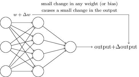
Learning algorithms are great. However, how to develop such an algorithm for a neural network? Suppose we have a network of perceptrons that we want to use to train the solution of the problem. Suppose the network's input can be pixels of a handwritten digit scanned image. And we want the network to know the weights and offsets necessary to properly classify numbers. To understand how this kind of training can work, let's imagine that we are changing a little bit of some weight (or offset) in the network. We want this small change to lead to a small change in the network output. As we soon see, this property makes learning possible. Schematically, we want the following (obviously, such a network is too simple to recognize handwriting!):



If a small change in weight (or displacement) would result in a small change in output, we could change the weights and offsets so that our network behaves a little closer to what we want. For example, suppose that the network incorrectly attributed the image to "8", although it should have been assigned to "9". We could figure out how to make a small change in weights and offsets, so that the network is a little closer to image classification, like “9”. And then we would repeat it, changing weights and shifts over and over again to get the best and best result. The network would learn.

The problem is that if there are perceptrons in the network, this does not happen. A small change in the weights or displacement of any perceptron can sometimes lead to a change in its output to the opposite, say, from 0 to 1. Such a revolution can change the behavior of the rest of the network in a very complex way. And even if now our “9” will be correctly recognized, the behavior of the network with all the other images is likely to have completely changed in a way that is difficult to control. Because of this, it is difficult to imagine how you can gradually adjust the weights and offsets so that the network gradually approaches the desired behavior. Perhaps there is some clever way around this problem. But there is no simple solution to the problem of learning the network of perceptrons.

This problem can be circumvented by introducing a new type of artificial neuron called the sigmoid neuron. They look like perceptrons, but are modified so that small changes in weights and offsets result in only small changes in the output. This is the main fact that will allow the network of sigmoid neurons to learn.

Let me describe the sigmoid neuron. We will draw them in the same way as perceptrons:



It also has input data x ₁ , x ₂ , ... But instead of being equated to 0 or 1, these inputs can have any value in the range from 0 to 1. K For example, a value of 0.638 would be a valid input for a sigmoid neuron (CH). Like the perceptron, CH has weights for each input, w ₁ , w₂ , ... and the total offset b. But its output value will not be 0 or 1. It will be σ (w⋅x + b), where σ is a sigmoid.

By the way, σ is sometimes called the logistic function , and this class of neurons is called logistic neurons. This terminology is useful to remember, as many people working with neural networks use these terms. However, we will stick to sigmoid terminology.

The function is defined as:

$$

$$\sigma(z) \equiv \frac{1}{1+e^{-z}} \tag{3}$$

In our case, the output value of the sigmoid neuron with input data x ₁ , x ₂ , ... weights w ₁ , w ₂ , ... and the offset b will be considered as:

$$

$$\frac{1}{1+exp(-\sum_j w_jx_j - b)} \tag{4}$$

At first glance, CH seem to be completely different from neurons. The algebraic form of sigmoids may seem confusing and obscure if you are not familiar with it. In fact, there are many similarities between perceptrons and CH, and the algebraic form of sigmoids turns out to be more technical in detail than a serious barrier to understanding.

To understand the similarity with the perceptron model, suppose that z ≡ w ⋅ x + b is a large positive number. Then e - z ≈ 0, therefore σ (z) ≈ 1. In other words, when z = w ⋅ x + b is large and positive, the output of CH is approximately equal to 1, as in the perceptron. Suppose that z = w ⋅ x + b is large with a minus sign. Then e - z → ∞, and σ (z) ≈ 0. So, for large z with a minus sign, the behavior of CH also approaches the perceptron. And only when w ⋅ x + b has an average size, serious deviations from the perceptron model are observed.

What about an algebraic form σ? How do we understand him? In fact, the exact form of σ is not so important - the form of the function on the graph is important. Here she is:



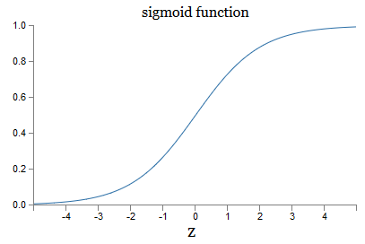
This is a smoothed version of the step function:



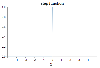
If σ were stepped, then CH would be a perceptron, since it would have 0 or 1 output depending on the sign w ⋅ x + b (well, in fact, at z = 0 the perceptron produces 0 , and the step function is 1, so that at one point, the function would have to be changed).

Using the real function σ, we obtain a smoothed perceptron. And the main thing here is the smoothness of the function, and not its exact form. Smoothness means that small changes in Δw _j weights and δb offsets will give small changes in Δoutput output. The algebra tells us that Δoutput is well approximated as follows:

$$

$$\Delta output \approx \sum_j \frac{\partial output}{\partial w_j}\Delta w_j + \frac{\partial output}{\partial b}\Delta b \tag{5}$$

Where the summation goes over all weights w _j , and ∂output / ∂w _j and ∂output / ∂b denote the partial derivatives of the output data on w _j and b, respectively. Do not panic if you feel insecure in the company of private derivatives! Although the formula looks complicated, with all these partial derivatives, it actually says something quite simple (and useful): Δoutput is a linear function depending on the Δw _j and Δb of the weights and the offset. Its linearity facilitates the selection of small changes in weights and offsets to achieve any desired small output offset. So, although in terms of their qualitative behavior, CHs are similar to perceptrons, they make it easier to understand how you can change the output by changing weights and offsets.

If the general form σ matters for us, and not its exact form, then why do we use just such a formula (3)? In fact, later we will sometimes consider neurons whose output is equal to f (w (x + b), where f () is some other activation function. The main thing that changes when changing a function is the values ​​of partial derivatives in equation (5). It turns out that when we then calculate these partial derivatives, the use of σ greatly simplifies algebra, since the exponentials have very pleasant properties when differentiating. In any case, σ is often used in work with neural networks, and most often in this book we will use such an activation function.

How to interpret the result of CH? Obviously, the main difference between perceptrons and CHs is that CHs do not give out only 0 or 1. Their output can be any real number from 0 to 1, so values ​​like 0.173 or 0.689 are valid. This can be useful, for example, if you need the output value to indicate, for example, the average brightness of the pixels of the image received at the input of the NA. But sometimes it can be uncomfortable. Suppose we want the network output to say that “image 9 has arrived at the input” or “incoming image is not 9”. Obviously, it would be easier if the output values ​​were 0 or 1, as in the perceptron. But in practice, we can agree that any output value not less than 0.5 would mean “9” at the input, and any value less than 0.5 would mean that it is “not 9”.I will always clearly indicate the existence of such arrangements.

Exercises

• SN simulating perceptrons, part 1

Suppose we take all the weights and offsets from the network of perceptrons, and multiply them by the positive constant c> 0. Show that the network behavior does not change.

• SN simulating perceptrons, part 2

Suppose we have the same situation as in the previous task - the network of perceptrons. Also assume that the input data is selected for the network. We do not need a specific value, the main thing is that it is fixed. Suppose the weights and displacements are such that w⋅x + b ≠ 0, where x is the input value of any perceptron of the network. Now we replace all perceptrons in the network by cN, and multiply the weights and displacements by a positive constant c> 0. Show that in the limit c → ∞, the behavior of the network from CH will be exactly the same as the network of perceptrons. How will this statement be violated if for one of the perceptrons w⋅x + b = 0?

Neural network architecture

In the next section, I will introduce a neural network capable of a good classification of handwritten numbers. Before that, it is useful to explain terminology that allows us to point to different parts of the network. Suppose we have the following network:



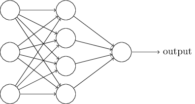
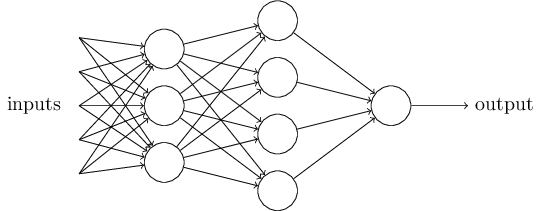
As I already mentioned, the leftmost layer in the network is called the input layer, and its neurons are called the input neurons. The rightmost, or output layer, contains the output neurons, or, as in our case, one output neuron. The middle layer is called hidden because its neurons are neither input nor output. The term "hidden" may sound a little mysterious - for the first time I heard it, I decided that it should have some deep philosophical or mathematical importance - but it means only "no entry and no exit." The network above has only one hidden layer, but some networks have several hidden layers. For example, in the following four-layer network there are two hidden layers:



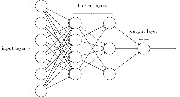
This can be confusing, but for historical reasons such networks with several layers are sometimes called multilayer perceptrons, MLP, despite the fact that they consist of sigmoid neurons rather than perceptrons. I am not going to use such terminology, since it is confusing, but I must warn of its existence.

Designing input and output layers is sometimes a simple task. For example, let's say we are trying to determine whether the handwritten number means “9” or not. A natural network circuit will encode the brightness of the image pixels in the input neurons. If the image is black and white, 64x64 pixels in size, then we will have 64x64 = 4096 input neurons, with a brightness in the range from 0 to 1. The output layer will contain only one neuron, whose value less than 0.5 will mean that “on the input was not 9 ", and the values ​​more will mean that" the input was 9 ".

And if the design of input and output layers is often a simple task, then the design of hidden layers can be a complicated art. In particular, it is impossible to describe the process of developing hidden layers with the help of a few simple practical rules. Researchers of the National Assembly have developed many heuristic rules for designing hidden layers to help get the desired behavior of neural networks. For example, such heuristics can be used to understand how to reach a compromise between the number of hidden layers and the time available for network training. Later we will come across some of these rules.

So far we have discussed NA, in which the output of one layer is used as input for the next. Such networks are called forward propagation neural networks. This means that there are no loops in the network - information always flows forward and never feeds back. If we had loops, we would have encountered situations in which the input data sigmoids would depend on the output. It would be hard to comprehend, and we do not allow such loops.

However, there are other models of artificial NA in which it is possible to use feedback loops. These models are called recurrent neural networks (RNS). The idea of ​​these networks is that their neurons are activated for limited periods of time. This activation can stimulate other neutrons, which can be activated a little later, also for a limited time. This leads to the activation of the following neurons, and over time we get a cascade of activated neurons. Loops in such models do not pose a problem, since the output of a neuron affects its entrance to some later point, and not immediately.

The RNS were not as influential as the direct propagation NA, in particular, because the training algorithms for the RNS so far have fewer capabilities. However, the PHC is still extremely interesting. In the spirit of the work they are much closer to the brain than the NA direct distribution. It is possible that the RNS will be able to solve important tasks that can be solved with great difficulty with the help of the ND. However, in order to limit the scope of our study, we will focus on more widely used NA direct distribution.

Simple handwriting classification network

Having determined the neural network, let us return to handwriting recognition. We can divide the task of recognizing handwritten numbers into two subtasks. First we want to find a way to split an image containing many digits into a sequence of separate images, each of which contains one digit. For example, we would like to break the image



into six separate



We, people, easily solve this segmentation problem, but for a computer program it is difficult to correctly split an image. After segmentation, the program needs to classify each individual digit. So, for example, we want our program to recognize that the first digit



this is 5.

We will focus on creating a program for solving the second task, the classification of individual numbers. It turns out that the segmentation task is not as difficult to solve as soon as we find a good way to classify individual numbers. To solve the problem of segmentation, there are many approaches. One of them is to try many different ways of image segmentation using a classifier of individual numbers, evaluating each attempt. Trial segmentation is highly appreciated if the classifier of individual numbers is confident in the classification of all segments, and low if it has problems in one or several segments. The idea is that if the classifier has problems somewhere, it most likely means that the segmentation is incorrect. This idea and other options can be used to solve the segmentation problem quite well. So, instead of worrying about segmentation, we will focus on developing an NA that can solve a more interesting and challenging task, namely, recognize individual handwritten numbers.

For the recognition of individual numbers, we will use the NA of three layers:



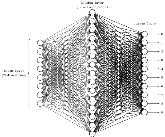
The input network layer contains neurons that encode different values ​​of the input pixels. As will be indicated in the next section, our training data will consist of a set of images of scanned handwritten numbers of 28x28 pixels, so the input layer contains 28x28 = 784 neurons. For simplicity, I did not specify most of the 784 neurons in the diagram. The incoming pixels are black and white, with a value of 0.0 indicating white, 1.0 indicating black, and intermediate values ​​indicating increasingly darker shades of gray.

The second layer of the network is hidden. We denote the number of neurons in this layer n, and we will experiment with different values ​​of n. The example above shows a small hidden layer containing only n = 15 neurons.

In the output layer of the network 10 neurons. If the first neuron is activated, that is, its output value is ≈ 1, this indicates that the network considers that the input was 0. If the second neuron is activated, the network considers that there was 1 at the input. And so on. Strictly speaking, we number the output neurons from 0 to 9, and see which one of them has the maximum activation value. If this is, let's say, neuron No. 6, then our network considers that the number 6 was at the input. And so on.

You may wonder why we need to use ten neurons. After all, we want to know which digit from 0 to 9 corresponds to the input image. It would be natural to use only 4 output neurons, each of which would take a binary value depending on whether its output value is closer to 0 or 1. Four neurons will be enough, since 2 ⁴ = 16, more than 10 possible values. Why should our network use 10 neurons? This is ineffective? The basis for this is empirical; we can try both versions of the network, and it turns out that for this task a network with 10 output neurons is better trained to recognize numbers than a network with 4. However, the question remains, why are 10 output neurons better? Is there any heuristics that would tell us in advance that you should use 10 output neurons instead of 4?

To understand why, it is useful to think about what makes a neural network. Consider first the variant with 10 output neurons. Let's concentrate on the first output neuron, which is trying to decide whether the incoming image is zero. He does this by weighing the evidence obtained from the hidden layer. What do hidden neurons do? Suppose the first neuron in the hidden layer determines whether there is something like this in the picture:



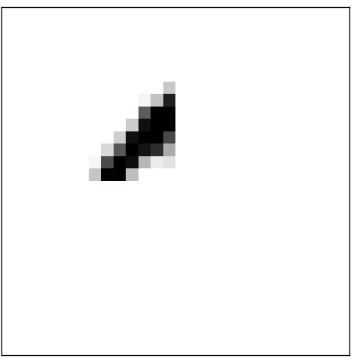
He can do this by assigning large weights to the pixels that coincide with this image, and small weights to the rest. In the same way, we assume that the second, third, and fourth neurons in the hidden layer are looking for whether there are such fragments in the image:



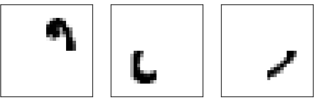
As you might have guessed, collectively, these four fragments give the image 0, which we saw earlier:



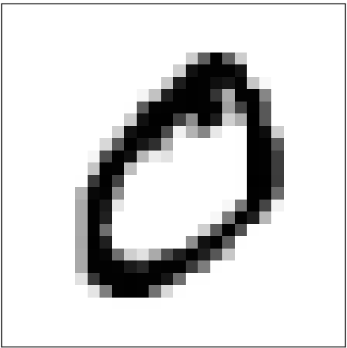
So, if four hidden neurons are activated, we can conclude that the number is 0. Of course, this is not the only evidence that 0 was shown there - we can get 0 and in many other ways (by slightly shifting these images or slightly distorting them). However, it can be said for sure that, at least in this case, we can conclude that the input was 0.

If we assume that the network works this way, we can give a plausible explanation for why it is better to use 10 output neurons instead of 4. If we had 4 output neurons, then the first neuron would try to decide what is the most significant bit of the incoming digit. And there is no easy way to associate the most significant bit with the simple forms given above. It is difficult to imagine any historical reasons for which parts of the form of the number would be somehow related to the most significant bit of the output data.

However, all of the above is supported only by heuristics. Nothing speaks in favor of the fact that the three-layer network should work as I said, and hidden neurons should find simple components of the forms. Perhaps a clever learning algorithm will find some weights that will allow us to use only 4 output neurons. However, as a heuristic, my method works well, and can save you considerable time in developing a good NA architecture.

Exercises

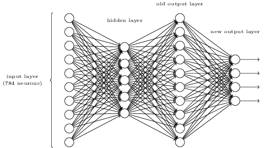
• There is a way to determine the bitwise representation of a number by adding an extra layer to the three-layer network. The additional layer converts the output values ​​of the previous layer to binary format, as shown in the figure below. Find the weights and offsets for the new output layer. We assume that the first 3 layers of neurons are such that the correct output from the third layer (the former output layer) is activated by values ​​of at least 0.99, and incorrect output values ​​do not exceed 0.01.

Gradient Descent Training

So, we have a NA scheme - how can she learn to recognize numbers? The first thing we need is training data, the so-called. training data set. We will use the MNIST set , containing tens of thousands of scanned images of handwritten numbers, and their correct classification. The name MNIST is due to the fact that it is a modified subset of the two data sets collected by NIST , the US National Institute of Standards and Technology. Here are some images from MNIST:



These are the same figures that were given at the beginning of the chapter as a recognition problem. Of course, when checking the NA, we will ask her to recognize the wrong images that were already in the training set!

MNIST data consists of two parts. The first contains 60,000 images intended for learning. This scanned handwritten notes of 250 people, half of whom were employees of the US Census Bureau, and the second half - high school students. Images are black and white, measuring 28x28 pixels. The second part of the MNIST dataset is 10,000 images to test the network. These are also black and white images of 28x28 pixels. We will use this data to assess how well the network has learned to recognize numbers. To improve the quality of the assessment, these figures were taken from another 250 people who did not participate in the enrollment (although these were also Bureau staff and high school students). This helps us to make sure that our system can recognize handwritten input of people that it has not met during the training.

We denote the training input by x. It will be convenient to treat each input image x as a vector with 28x28 = 784 dimensions. Each value inside the vector indicates the brightness of one pixel of the image. The output value will be denoted as y = y (x), where y is a ten-dimensional vector. For example, if a specific training image x contains 6, then y (x) = (0,0,0,0,0,0,0,0,0,0) ^T will be the vector we need. T is a transpose operation that turns a row vector into a column vector.

We want to find an algorithm that allows us to search for such weights and displacements so that the output of the network approaches y (x) for all training inputs x. To quantify the approximation to this goal, we define the cost function (sometimes called the loss function ; in the book we will use the cost function, but keep in mind another name):

$$

$$C (w, b) = \ frac {1} {2n} \ sum_x || y (x) - a || ^ 2 \ tag {6}$$

Here w denotes a set of weights of the network, b is the set of offsets, n is the number of training inputs, a is the output data vector, when x is the input data, and the sum goes through all the training input data x. The output, of course, depends on x, w and b, but for simplicity I did not denote this dependence. Designation || v || means the length of the vector v. We will call C a quadratic cost function; it is sometimes also referred to as root-mean-square error, or MSE. If you look at C, you can see that it is not negative, since all terms of the sum are non-negative. In addition, the cost C (w, b) becomes small, that is, C (w, b) ≈ 0, precisely when y (x) is approximately equal to the output vector a of all the training input data x. So our algorithm worked well, if it managed to find weights and offsets such that C (w, b) ≈ 0. And vice versa, it worked badly when C (w, b) is large - this means that y (x) does not match with output for a large amount of input data. It turns out that the purpose of the learning algorithm is to minimize the cost of C (w, b) as a function of weights and offsets. In other words, we need to find a set of weights and offsets that minimizes the value of the cost. We will do this with an algorithm called gradient descent.

Why do we need a quadratic cost? Are we not mainly interested in the number of images correctly recognized by the network? Is it possible to simply maximize this number directly, and not to minimize the intermediate value of the quadratic value? The problem is that the number of correctly recognized images is not a smooth function of the weights and network offsets. For the most part, small changes in weights and offsets will not change the number of correctly recognized images. Because of this, it is hard to understand how to change weights and biases to improve efficiency. If we use the smooth cost function, it will be easy for us to understand how to make small changes in weight and displacement to improve the cost. Therefore, we first concentrate on the quadratic cost, and then we will examine the accuracy of the classification.

Even considering that we want to use a smooth cost function, you can still wonder - why did we choose the quadratic function for equation (6)? Can it not be chosen arbitrarily? Perhaps if we chose a different function, we would get a completely different set of minimizing weights and offsets. A reasonable question, and later we will again study the cost function and make some edits to it. However, the quadratic cost function works great for understanding basic things in NA learning, so for now we’ll stick to it.

To summarize: our goal in teaching NN comes down to finding weights and displacements that minimize the quadratic cost function C (w, b). The task is well set, but so far it has many distracting structures - interpreting w and b as weights and offsets, function σ hidden in the background, choice of network architecture, MNIST, and so on. It turns out that we can understand a great deal, ignoring most of this structure, and concentrating only on the aspect of minimization. So for the time being, we will forget about the special form of the cost function, communication with NA and so on. Instead, we are going to imagine that we simply have a function with many variables, and we want to minimize it. We will develop a technology called gradient descent, which can be used to solve such problems. And then we will return to a certain function that we want to minimize for the National Assembly.

Well, let's say we are trying to minimize a certain function C (v). It can be any function with real values ​​in many variables v = v ₁ , v ₂ , ... Notice that I replaced the entry w and b with v, to show that it can be any function - we are no longer fixating on the NA. It is useful to imagine that the C function has only two variables - v ₁ and v ₂ :



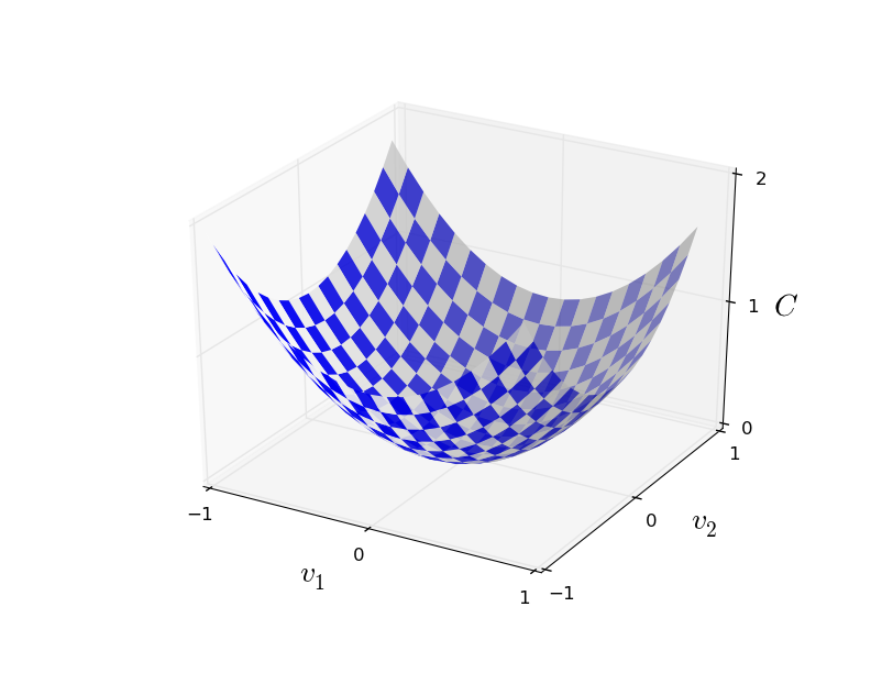
We would like to find where C reaches the global minimum. Of course, with the function drawn above, we can study the graph and find the minimum. In this sense, I may have given you a function too simple! In general, C can be a complex function of many variables, and it is usually impossible to just look at the graph and find the minimum.

One of the ways to solve the problem is to use algebra to find the minimum analytically. We can calculate the derivatives and try to use them to find the extremum. If we are lucky, it will work when C is a function of one or two variables. But with a large number of variables, this turns into a nightmare. And for NA, we often need much more variables — for the largest NA, the cost functions in a complex way depend on billions of weights and offsets. Use algebra to minimize these functions will not work!

(Having said that it would be more convenient for us to consider C as a function of two variables, I twice in two paragraphs said “yes, but what if it is a function of a much larger number of variables?” I apologize. Believe that it would be useful for us to represent C as a function two variables. Sometimes this picture falls apart, which is why the two previous sections were needed. For mathematical reasoning, it is often necessary to juggle with several intuitive representations, learning when the presentation can be used, and when not zya.)

Okay, so algebra won't work. Fortunately, there is a great analogy that suggests a well-functioning algorithm. We see our function as something of a valley. With the latest schedule it will not be so difficult to do. And we imagine a ball rolling down the side of a valley. Our experience tells us that the ball will eventually roll to the bottom. Perhaps we can use this idea to find the minimum of a function? We will randomly choose the starting point for an imaginary ball, and then simulate the movement of the ball, as if it were rolling down to the bottom of a valley. We can use this simulation simply by counting the derivatives (and, possibly, the second derivatives) C - they will tell us everything about the local form of the valley, and, consequently, about how our ball will roll.

Based on what you have written, you might think that we will write down Newton's equations of motion for the ball, consider the effects of friction and gravity, and so on. In fact, we will not follow this analogy with the ball so closely - we are developing an algorithm for minimizing C, and not an exact simulation of the laws of physics! This analogy should stimulate our imagination, and not limit thinking. So instead of diving into the complex details of physics, let's ask the question: if we were appointed by God for one day, and we would create our own laws of physics, telling the ball how to roll which law or laws of motion we would choose so that the ball always rolls on valley bottom?

To clarify the question, let's think about what happens if we move the ball a small distance Δv ₁ in the direction of v ₁, and a small distance Δv ₂ in the direction of v ₂ . Algebra tells us that C changes as follows:

$$

$$\Delta C \approx \frac{\partial C}{\partial v_1} \Delta v_1 + \frac{\partial C}{\partial v_2} \Delta v_2 \tag{7}$$

We will find a way to select Δv ₁ and Δv ₂ such that ΔC is less than zero; that is, we will select them so that the ball rolls down. To understand how to do this, it is useful to define Δv as a vector of changes, that is, Δv ≡ (Δv ₁ , Δv ₂ ) ^T , where T is the transpose operation that turns the row vectors into column vectors. We also define the gradient vector C as partial derivatives (∂S / ∂v ₁ , ∂S / ∂v ₂ ) ^T . Denote the gradient vector, we will ∇C:

$$

$$\nabla C \equiv (\frac{\partial C}{\partial v_1}, \frac{\partial C}{\partial v_2})^T \tag{8}$$

Soon we will rewrite the change in ΔC through Δv and gradient C. In the meantime, I want to clarify something, which is why people often hang on the gradient. When they first meet C, people sometimes don’t understand how they should perceive the symbol. What does he specifically mean? In fact, you can safely assume that C is a single mathematical object — a vector previously defined — that is simply written using two characters. From this point of view, ∇ is like waving a flag telling that "∇C is a gradient vector." There are also more advanced points of view, from which ∇ can be considered as an independent mathematical entity (for example, as a differentiation operator), but we will not need them.

With such definitions, expression (7) can be rewritten as:

$$

$$\Delta C \approx \nabla C \cdot \Delta v \tag{9}$$

This equation helps explain why ∇C is called a gradient vector: it associates changes in v with changes in C, exactly as expected from an entity called a gradient. [eng gradient - deviation / approx. transl.] However, it is more interesting that this equation allows us to see how to choose Δv so that ΔC is negative. Let's say we choose

$$

$$\Delta v = - \eta \nabla C \tag{10}$$

where η is a small positive parameter (learning rate). Then equation (9) tells us that ΔC & approx; - η ∇C & cdot; = - η || ∇C || ²Since || ∇C || ² ≥ 0, this ensures that ΔC ≤ 0, that is, C will decrease all the time if we change v, as stated in (10) (of course, within the approximation from equation (9)). And that is exactly what we need! Therefore, we take equation (10) to determine the "law of motion" of the ball in our gradient descent algorithm. That is, we will use equation (10) to calculate the value of Δv, and then we will move the ball to this value:

$$

$$v \rightarrow v' = v - \eta \nabla C \tag{11}$$

Then we again apply this rule for the next move. Continuing the repetition, we will lower C until, as we hope, we reach a global minimum.

Summing up, the gradient descent works through the sequential calculation of the gradient ∇ C, and the subsequent displacement in the opposite direction, which leads to a “fall” along the slope of the valley. This can be visualized as follows:



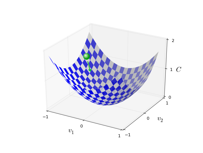
Note that with this rule, gradient descent does not reproduce real physical movement. In real life, the ball has an impulse that can allow it to roll across a slope, or even roll up for a while. Only after the work of the friction force the ball is guaranteed to roll down the valley. Our selection rule, Δv, simply says “go down.” Pretty good rule for finding the minimum!

In order for the gradient descent to work correctly, we need to choose a sufficiently small value of the learning speed η so that equation (9) is a good approximation. Otherwise, it may turn out that ΔC> 0 is no good! At the same time, it is not necessary that η be too small, since then the changes in Δv will be tiny, and the algorithm will work too slowly. In practice, η changes in such a way that equation (9) gives a good approximation, and the algorithm did not work too slowly. We will see later how this works.

I explained the gradient descent, when function C depended only on two variables. But it works the same if C is a function of many variables. Suppose that it has m variables, v ₁ , ..., v _m. Then the change in ΔC caused by a small change in Δv = (Δv ₁ , ..., Δv _m ) ^T will equal

$$

$$\Delta C \approx \nabla C \cdot \Delta v \tag{12}$$

where the ∇C gradient is a vector

$$

$$\nabla C \equiv (\frac{\partial C}{\partial v_1},…, \frac{\partial C}{\partial v_m})^T \tag{13}$$

As with the two variables, we can choose

$$

$$\Delta v = - \eta \nabla C \tag{14}$$

and ensure that our approximate expression (12) for ΔC is negative. This gives us a way to follow the gradient to a minimum, even when C is a function of many variables, applying the update rule over and over again.

$$

$$v \rightarrow v' = v - \eta \nabla C \tag{15}$$

This update rule can be considered the determining algorithm for gradient descent. It gives us the method of repeatedly changing the position of v in search of a minimum of function C. This rule does not always work - several things can go wrong by preventing the gradient descent from finding the global minimum C - by this point we will return in the following chapters. But in practice, gradient descent often works very well, and we will see that in NA it is an effective way to minimize the cost function, and, therefore, network training.

In a sense, gradient descent can be considered the optimal strategy for finding a minimum. Suppose we are trying to move Δv to the position to maximize C. This is equivalent to minimizing ΔC & approx; ∇C & cdot; Δv. We will limit the step size so that || Δv || = ε for some small constant ε> 0. In other words, we want to move a small distance of a fixed size, and try to find the direction of movement that reduces C as much as possible. It can be proved that choosing Δv that minimizes ∇C & cdot; Δv, equal to Δv = -η∇C, where η = ε / || ∇C ||, is determined by the constraint || Δv || = ε. So, gradient descent can be considered a way to take small steps in the direction that most strongly reduces C.

Exercises

• . : — , , , .
• , , . , ? ?

People have studied many options for gradient descent, including those that more accurately reproduce the real physical ball. Such options have their advantages, but also a big drawback: the need to calculate the second partial derivatives of C, which can take a lot of resources. To understand this, suppose that we need to calculate all the second partial derivatives of ∂ ² C / ∂ v _j ∂ v _k . If there are v _j million variables , then we need to calculate approximately a trillion (million squared) second partial derivatives (actually, half a trillion, since ∂ ² C / ∂ v _j ∂ v _k = ∂ ² C / v _k ∂ v _j. But you caught the essence). This will require a lot of computational resources. There are tricks to avoid this, and the search for alternatives to gradient descent is an area of ​​active research. However, in this book we will use gradient descent and its variants as the main approach to the teaching of the National Assembly.

How do we apply gradient descent to learning NA? We need to use it to search for weights w _k and displacements b _l minimizing the cost equation (6). Let's rewrite the update rule for gradient descent, replacing the variables v _{j with} weights and offsets. In other words, now our “position” has components w _k and b _l , and the gradient vector ∇C has corresponding components ∂C / ∂w_k and ∂C / ∂b _l . By writing our update rule with new components, we get:

$$

$$w_k \rightarrow w'_k = w_k - \eta \frac{\partial C}{\partial w_k} \tag{16}$$

$$

$$b_l \rightarrow b'_l = b_l - \eta \frac{\partial C}{\partial b_l} \tag{17}$$

By reapplying this update rule, we can “roll downhill” and, if we are lucky, find the minimum cost function. In other words, this rule can be used for teaching NA.

There are several obstacles to the application of the gradient descent rule. We will study them in more detail in the following chapters. But for now, I want to mention only one problem. To understand it, let's go back to the quadratic value in equation (6). Note that this cost function looks like C = 1 / n ∑ _x C _x , that is, it is an average of cost C _x (|| y (x) −a || ² ) / 2 for individual teaching examples. In practice, to calculate the gradient ∇C we need to calculate the gradients ∇C _xseparately for each training input x, and then averaging them, ∇C = 1 / n ∑ _x ∇C _x . Unfortunately, when the amount of input data is very large, it will take a very long time, and such training will take place slowly.

To speed up learning, you can use stochastic gradient descent. The idea is to approximate the gradient of ∇C by calculating ∇C _x for a small random sample of training input. Having considered their average, we can quickly get a good estimate of the true gradient of ∇C, and this helps speed up the gradient descent, and therefore learning.

More precisely, stochastic gradient descent works through random sampling of a small amount of m training input. We call this random data X ₁ , X ₂ , .., X _m , and call it a mini-packet. If the sample size m is large enough, the average value of ∇C _{X j} will be close enough to the average for all ∇Cx, that is,

$$

$$\frac{\sum^m_{j=1} \nabla C_{X_j}}{m} \approx \frac{\sum_x \nabla C_x}{n} = \nabla C \tag{18}$$

where the second amount goes across the entire training data set. Swapping the parts, we get

$$

$$\nabla C \approx \frac{1}{m} \sum^m_{j=1} \nabla C_{X_j} \tag{19}$$

which confirms that we can estimate the overall gradient by calculating gradients for a randomly selected mini-packet.

To relate this directly to the teaching of the NA, let's assume that w _k and b _l denote the weights and displacements of our NA. Then the stochastic gradient descent selects a random mini-packet of input data, and learns from them.

$$

$$w_k \rightarrow w'_k = w_k - \frac{\eta}{m} \sum_j \frac{\partial C_{X_j}}{\partial w_k} \tag{20}$$

$$

$$b_l \rightarrow b'_l = b_l - \frac{\eta}{m} \sum_j \frac{\partial C_{X_j}}{\partial b_l} \tag{21}$$

where is the summation of all teaching examples X _j in the current mini-package. Then we select another random mini-pack and learn from it. And so on, until we have exhausted all the training data, which is called the end of the learning era. At this moment we are starting a new era of learning.

By the way, it is worth noting that agreements regarding the scaling of the cost function and the updates of weights and offsets by the mini-package differ. In equation (6), we scaled the cost function by 1 / n times. Sometimes people omit 1 / n, summing up the cost of individual teaching examples, instead of calculating the average. This is useful when the total number of training examples is not known in advance. This can happen, for example, when additional data appears in real time. In the same way, the update rules for the mini-package (20) and (21) sometimes omit the 1 / m term before the sum. Conceptually, this does not affect anything, since it is equivalent to a change in the learning rate η. However, it is worth paying attention to when comparing different works.

A stochastic gradient descent can be thought of as a political vote: it is much easier to take a sample in the form of a mini-package than to apply a gradient descent to a full sample — just like a poll at the exit of a site is easier than conducting full choices. For example, if our training set has a size of n = 60,000, as MNIST, and we will sample a mini packet of size m = 10, then it will speed up the gradient estimation by a factor of 6000! Of course, the estimate will not be perfect - there will be a statistical fluctuation in it - but it doesn’t have to be perfect: we only need to move in approximately the direction that C decreases, which means that we don’t need to accurately calculate the gradient. In practice, stochastic gradient descent is a common and powerful teaching technique of the National Assembly, and the base of most of the training technologies that we develop in the framework of the book.

Exercises

• - 1. , x w _k → w′ _k = w _k − η ∂C _x / ∂w _k b _l → b′ _l = b _l − η ∂C _x / ∂b _l . . And so on. , -, . - ( ). - - 20.

Let us end this section with a discussion of a topic that sometimes worries people who first came across a gradient descent. In HC, cost C is a function of many variables — all weights and displacements — and in a sense, defines a surface in a very multidimensional space. People begin to think: “I will have to visualize all these extra dimensions.” And they begin to worry: “I cannot navigate in four dimensions, not to mention five (or five million)”. Do they not have any special quality available to the "real" supermathematicians? Of course not. Even professional mathematicians cannot visualize 4-dimensional space well enough — if they can at all. They go on tricks, developing other ways of presenting what is happening. We did just that:we used the algebraic (and not visual) representation of ΔC to understand how to move, so that C decreases. People who cope well with a large number of dimensions have a large library of similar techniques in their minds; our algebraic trick is just one example. These techniques may not be as simple as we are used to when visualizing three dimensions, but when you created a library of similar techniques, you start thinking well in higher dimensions. I will not go into details, but if you are interested, you might liketo which we are accustomed to visualizing three dimensions, but when you created a library of similar techniques, you begin to think well in higher dimensions. I will not go into details, but if you are interested, you might liketo which we are accustomed to visualizing three dimensions, but when you created a library of similar techniques, you begin to think well in higher dimensions. I will not go into details, but if you are interested, you might likediscussion of some of these techniques by professional mathematicians who are used to thinking in higher dimensions. And although some of the techniques discussed are quite complex, most of the best answers are intuitive and accessible to all.

Network implementation to classify numbers

Ok, now let's write a program that learns how to recognize handwritten numbers using stochastic gradient descent and MNIST training data. We will do this with a short python 2.7 program consisting of only 74 lines! The first thing we need is to download the MNIST data. If you use git, then you can get them by cloning the repository of this book:

git clone https://github.com/mnielsen/neural-networks-and-deep-learning.git

If not, download the code by reference .

By the way, when I mentioned the MNIST data before, I said that they are broken up into 60,000 training images and 10,000 verification images. This is the official description from MNIST. We will break the data a little differently. We will leave the verification images unchanged, but we will break the training set into two parts: 50,000 pictures, which we will use to train the National Assembly, and a separate 10,000 pictures for additional ratification. For the time being we will not use them, but later they will be useful to us when we understand the setting up of some hyperparameters of the National Assembly — learning rates, etc., which our algorithm does not directly choose. Although the ratification data is not included in the original MNIST specification, many people use MNIST in this way, and in the field of NA, the use of ratification data is common. Now, speaking of the “MNIST tutorial data,” I will refer to our 50,000 caritsnacks, not the original 60,000.

In addition to the MNIST data, we also need a python library called Numpy for quick calculations of linear algebra. If you do not have it, you can take it by reference .

Before giving you the whole program, let me explain the main features of the code for the NA. The central place is occupied by the Network class, which we use to represent the National Assembly. Here is the initialization code for the Network object:

 class Network(object): def __init__(self, sizes): self.num_layers = len(sizes) self.sizes = sizes self.biases = [np.random.randn(y, 1) for y in sizes[1:]] self.weights = [np.random.randn(y, x) for x, y in zip(sizes[:-1], sizes[1:])] 

The sizes array contains the number of neurons in the corresponding layers. So, if we want to create a Network object with two neurons in the first layer, three neurons in the second layer, and one neuron in the third, then we write it this way:

 net = Network([2, 3, 1]) 

Offsets and weights in the Network object are initialized randomly using the np.random.randn function from Numpy, which generates a Gaussian distribution with a mean of 0 and a standard deviation of 1. This random initialization gives our stochastic gradient descent algorithm a starting point. In the following chapters we will find the best ways to initialize weights and offsets, but for now this is enough. Note that the Network initialization code assumes that the first layer of neurons will be input, and does not assign displacements to them, since they are used only when calculating the output data.

Also note that offsets and weights are stored as an array of Numpy matrices. For example, net.weights [1] is a Numpy matrix that stores the weights connecting the second and third layers of neurons (this is not the first and second layers, since in python the numbering of the elements of the array comes from scratch). Since writing net.weights [1] will be too long, we denote this matrix as w. This is such a matrix that w _jk is the weight of the connection between the kth neuron in the second layer and the jth neuron in the third. Such an order of indices j and k may seem strange - would it not be more logical to swap them? But the big advantage of such a recording is that the activation vector of the third layer of neurons is obtained:

$$

$$a '= \ sigma (wa + b) \ tag {22}$$

Let's look at this rather saturated equation. a is the vector of activations of the second layer of neurons. To get a ', we multiply a by the weights matrix w, and add the displacement vector b. Then we apply the sigmoid σ elementwise to each element of the vector wa + b (this is called the vectorization of the function σ). It is easy to verify that equation (22) gives the same result as rule (4) for calculating the sigmoid neuron.

Exercise

• Write equation (22) in component form, and make sure that it gives the same result as rule (4) for calculating the sigmoid neuron.

Given all this, it is easy to write code that computes the output of a Network object. We begin by defining sigmoids:

 def sigmoid(z): return 1.0/(1.0+np.exp(-z)) 

Note that when the parameter z is a vector or an array of Numpy, then Numpy will automatically apply sigmoid elementwise, that is, in a vector form.

Add a direct distribution method to the Network class, which accepts input a from the network and returns the corresponding output. It is assumed that the a parameter is (n, 1) Numpy ndarray, and not a vector (n,). Here n is the number of input neurons. If you try to use a vector (n,), you will get strange results.

The method simply applies equation (22) to each layer:

  def feedforward(self, a): """       "a"""" for b, w in zip(self.biases, self.weights): a = sigmoid(np.dot(w, a)+b) return a 

Of course, most of us from Network objects need them to learn. To do this, we give them the SGD method that implements a stochastic gradient descent. Here is his code. In some places it is quite mysterious, but below we will analyze it in more detail.

  def SGD(self, training_data, epochs, mini_batch_size, eta, test_data=None): """    -    . training_data –   "(x, y)",       .       .  test_data ,          ,     .     ,    . """ if test_data: n_test = len(test_data) n = len(training_data) for j in xrange(epochs): random.shuffle(training_data) mini_batches = [ training_data[k:k+mini_batch_size] for k in xrange(0, n, mini_batch_size)] for mini_batch in mini_batches: self.update_mini_batch(mini_batch, eta) if test_data: print "Epoch {0}: {1} / {2}".format( j, self.evaluate(test_data), n_test) else: print "Epoch {0} complete".format(j) 

training_data is a list of "(x, y)" tuples denoting the training input and the desired output. The variables epochs and mini_batch_size are the number of epochs for training and the size of mini-packages for use. eta is the learning rate, η. If test_data is specified, then the network will be evaluated against the verification data after each epoch, and the current progress will be displayed. This is useful for tracking progress, but slows down significantly.

The code works like this. In each epoch, he begins by randomly mixing the training data, and then splitting them into mini packets of the desired size. This is an easy way to create a sample of training data. Then for each mini_batch we apply one step gradient descent. This makes the code self.update_mini_batch (mini_batch, eta) updating the weights and offsets of the network according to one iteration of the gradient descent, using only the training data in mini_batch. Here is the code for the update_mini_batch method:

  def update_mini_batch(self, mini_batch, eta): """    ,          -. mini_batch –    (x, y),  eta –  .""" nabla_b = [np.zeros(b.shape) for b in self.biases] nabla_w = [np.zeros(w.shape) for w in self.weights] for x, y in mini_batch: delta_nabla_b, delta_nabla_w = self.backprop(x, y) nabla_b = [nb+dnb for nb, dnb in zip(nabla_b, delta_nabla_b)] nabla_w = [nw+dnw for nw, dnw in zip(nabla_w, delta_nabla_w)] self.weights = [w-(eta/len(mini_batch))*nw for w, nw in zip(self.weights, nabla_w)] self.biases = [b-(eta/len(mini_batch))*nb for b, nb in zip(self.biases, nabla_b)] 

Most of the work is done by the line.

  delta_nabla_b, delta_nabla_w = self.backprop(x, y) 

It triggers backpropagation algorithm — it's a quick way to calculate the gradient of the cost function. So update_mini_batch simply calculates these gradients for each tutorial from mini_batch, and then updates self.weights and self.biases.

So far, I will not demonstrate the code for self.backprop. We will study back propagation work in the next chapter, and there will be self.backprop code. For now, suppose that it behaves, as stated, by returning the appropriate gradient for the cost associated with teaching example x.

Let's look at the program entirely, including explanatory comments. With the exception of the self.backprop function, the program speaks for itself - the main work is done by self.SGD and self.update_mini_batch. The self.backprop method uses several additional functions to calculate the gradient, namely, sigmoid_prime, which calculates the sigmoid derivative, and self.cost_derivative, which I will not describe here. You can get an idea of ​​them by reviewing the code and comments. In the next chapter we will look at them in more detail. Note that although the program seems to be long, most of the code is comments that facilitate understanding. In fact, the program itself consists of only 74 lines of code — not empty and no comments. All code is available on GitHub .

 """ network.py ~~~~~~~~~~           .      .     ,    .   ,       . """ ####  #   import random #   import numpy as np class Network(object): def __init__(self, sizes): """  sizes      .  ,      Network      ,     ,     ,    ,  [2, 3, 1].               0    1. ,      ,       ,        . """ self.num_layers = len(sizes) self.sizes = sizes self.biases = [np.random.randn(y, 1) for y in sizes[1:]] self.weights = [np.random.randn(y, x) for x, y in zip(sizes[:-1], sizes[1:])] def feedforward(self, a): """   ,  ``a`` -  .""" for b, w in zip(self.biases, self.weights): a = sigmoid(np.dot(w, a)+b) return a def SGD(self, training_data, epochs, mini_batch_size, eta, test_data=None): """    -    . training_data –   "(x, y)",       .       .  test_data ,          ,     .     ,    . """ if test_data: n_test = len(test_data) n = len(training_data) for j in xrange(epochs): random.shuffle(training_data) mini_batches = [ training_data[k:k+mini_batch_size] for k in xrange(0, n, mini_batch_size)] for mini_batch in mini_batches: self.update_mini_batch(mini_batch, eta) if test_data: print "Epoch {0}: {1} / {2}".format( j, self.evaluate(test_data), n_test) else: print "Epoch {0} complete".format(j) def update_mini_batch(self, mini_batch, eta): """    ,          -. mini_batch –    (x, y),  eta –  .""" nabla_b = [np.zeros(b.shape) for b in self.biases] nabla_w = [np.zeros(w.shape) for w in self.weights] for x, y in mini_batch: delta_nabla_b, delta_nabla_w = self.backprop(x, y) nabla_b = [nb+dnb for nb, dnb in zip(nabla_b, delta_nabla_b)] nabla_w = [nw+dnw for nw, dnw in zip(nabla_w, delta_nabla_w)] self.weights = [w-(eta/len(mini_batch))*nw for w, nw in zip(self.weights, nabla_w)] self.biases = [b-(eta/len(mini_batch))*nb for b, nb in zip(self.biases, nabla_b)] def backprop(self, x, y): """  ``(nabla_b, nabla_w)``,      C_x. ``nabla_b``  ``nabla_w`` -    numpy,   ``self.biases`` and ``self.weights``.""" nabla_b = [np.zeros(b.shape) for b in self.biases] nabla_w = [np.zeros(w.shape) for w in self.weights] #   activation = x activations = [x] #      zs = [] #     z- for b, w in zip(self.biases, self.weights): z = np.dot(w, activation)+b zs.append(z) activation = sigmoid(z) activations.append(activation) #   delta = self.cost_derivative(activations[-1], y) * \ sigmoid_prime(zs[-1]) nabla_b[-1] = delta nabla_w[-1] = np.dot(delta, activations[-2].transpose()) """ l      ,      . l = 1    , l = 2 – ,   .    ,   python      .""" for l in xrange(2, self.num_layers): z = zs[-l] sp = sigmoid_prime(z) delta = np.dot(self.weights[-l+1].transpose(), delta) * sp nabla_b[-l] = delta nabla_w[-l] = np.dot(delta, activations[-l-1].transpose()) return (nabla_b, nabla_w) def evaluate(self, test_data): """    ,      .    –          .""" test_results = [(np.argmax(self.feedforward(x)), y) for (x, y) in test_data] return sum(int(x == y) for (x, y) in test_results) def cost_derivative(self, output_activations, y): """    ( C_x /  a)   .""" return (output_activations-y) ####   def sigmoid(z): """.""" return 1.0/(1.0+np.exp(-z)) def sigmoid_prime(z): """ .""" return sigmoid(z)*(1-sigmoid(z)) 

How well does the program recognize handwritten numbers? Let's start by loading the MNIST data. We do this with a small helper program mnist_loader.py, which I will describe below. Run the following commands in the python shell:

 >>> import mnist_loader >>> training_data, validation_data, test_data = \ ... mnist_loader.load_data_wrapper() 

This, of course, can be done in a separate program, but if you work in parallel with the book, it will be easier.

After downloading the MNIST data, we set up a network of 30 hidden neurons. We will do this after importing the program described above, which is called network:

 >>> import network >>> net = network.Network([784, 30, 10]) 

Finally, we use a stochastic gradient descent for training on training data for 30 epochs, with a mini-packet size of 10, and a learning rate of η = 3.0:

 >>> net.SGD(training_data, 30, 10, 3.0, test_data=test_data) 

If you execute code in parallel with reading a book, please note that it will take several minutes to complete. I suggest you run everything, continue reading, and periodically check what the program gives out. If you are in a hurry, you can reduce the number of epochs by reducing the number of hidden neurons, or using only a fraction of the training data. The final working code will work faster: these python scripts are designed to make you understand how the network works, and they are not high-performance! And, of course, after training, the network can work very quickly on almost any computing platform. For example, when we teach the network a good set of weights and offsets, it can easily be ported to work in JavaScript in a web browser, or as a native application on a mobile device. In any case, about such a conclusion gives a program that teaches a neural network. She writes the number of correctly recognized test images after each training era. As you can see, even after one epoch, it reaches an accuracy of 9,129 out of 10,000, and this number continues to grow:

Epoch 0: 9129 / 10000
Epoch 1: 9295 / 10000
Epoch 2: 9348 / 10000
...
Epoch 27: 9528 / 10000
Epoch 28: 9542 / 10000
Epoch 29: 9534 / 10000

It turns out that a trained network gives a percentage of correct classification of about 95 - 95.42% at the maximum! Quite a promising first attempt. I warn you that your code will not necessarily produce exactly the same results, since we initialize the network with random weights and offsets. For this chapter, I chose the best of the three attempts.

Let's restart the experiment by changing the number of hidden neurons to 100. As before, if you run the code simultaneously with reading, note that it takes quite a long time to complete (on my machine, each epoch takes several tens of seconds), so it’s best to read in parallel with the execution code.

 >>> net = network.Network([784, 100, 10]) >>> net.SGD(training_data, 30, 10, 3.0, test_data=test_data) 

Naturally, this improves the result to 96.59%. At least in this case, using more hidden neurons helps to get better results.

Feedback from readers suggests that the results of this experiment vary greatly, and some of the learning outcomes are much worse. Using techniques from Chapter 3 will seriously reduce the variety of work efficiency from one run to the next.

Of course, in order to achieve such accuracy, I had to choose a certain number of epochs for learning, a mini-packet size and a learning rate η. As I mentioned above, they are called the hyperparameters of our NA — to distinguish them from simple parameters (weights and offsets) that the algorithm sets up in the learning process. If we choose poorly hyper parameters, we will get poor results. Suppose, for example, that we chose the learning rate η = 0.001:

 >>> net = network.Network([784, 100, 10]) >>> net.SGD(training_data, 30, 10, 0.001, test_data=test_data) 

The results are much less impressive:

Epoch 0: 1139 / 10000
Epoch 1: 1136 / 10000
Epoch 2: 1135 / 10000
...
Epoch 27: 2101 / 10000
Epoch 28: 2123 / 10000
Epoch 29: 2142 / 10000

However, it can be seen that network efficiency is slowly growing over time. This suggests that you can try to increase the speed of learning, for example, to 0.01. In this case, the results will be better, which suggests the need to further increase the speed (if the change improves the situation, change further!). If you do this several times, we end up with η = 1.0 (and sometimes even 3.0), which is close to our earlier experiments. So, although we initially poorly selected hyper parameters, at least we collected enough information to be able to improve our choice of parameters.

In general, debugging NA is difficult. This is especially so when the choice of initial hyperparameters produces results that do not exceed the random noise. Suppose we try to use a successful architecture of 30 neurons, but change the learning speed to 100.0:

 >>> net = network.Network([784, 30, 10]) >>> net.SGD(training_data, 30, 10, 100.0, test_data=test_data) 

In the end, it turns out that we have gone too far, and took too much speed:

Epoch 0: 1009 / 10000
Epoch 1: 1009 / 10000
Epoch 2: 1009 / 10000
Epoch 3: 1009 / 10000
...
Epoch 27: 982 / 10000
Epoch 28: 982 / 10000
Epoch 29: 982 / 10000

Now imagine that we are approaching this task for the first time. Of course, we know from early experiments that it would be correct to reduce the speed of learning. But if we were to approach this task for the first time, we would have no output that could lead us to the right decision. Could we start thinking that maybe we chose the wrong starting parameters for weights and offsets, and the network is difficult to learn? Or perhaps we don’t have enough training data to get a meaningful result? Perhaps we did not wait for enough eras? Perhaps a neural network with such an architecture simply cannot learn to recognize handwritten numbers? Perhaps the learning rate is too low? The first approach to the problem you never have confidence.

From this it is worthwhile to learn the lesson that debugging NA is not a trivial task, and this, like ordinary programming, is part of art. You need to learn this debugging art to get good results from the NA. In general, we need to develop heuristics for choosing good hyperparameters and good architecture. We will discuss this in detail in the book, including how I chose the above hyperparameters.

Exercise

• Try to create a network of just two layers - input and output, without hidden - with 784 and 10 neurons, respectively. Teach the net with a stochastic gradient descent. What classification accuracy do you get?

Earlier, I missed the details of loading MNIST data. It happens quite simply. Here is the code for completeness. The data structures are described in the comments - everything is simple, the tuples and arrays of Numpy ndarray objects (if you are not familiar with such objects, imagine them as vectors).

 """ mnist_loader ~~~~~~~~~~~~      MNIST.       ``load_data``  ``load_data_wrapper``.  , ``load_data_wrapper`` -  ,     . """ ####  #  import cPickle import gzip #  import numpy as np def load_data(): """  MNIST   ,  ,    . ``training_data``      .    .  numpy ndarray  50 000 .   –     numpy ndarray  784 ,  28 * 28 = 784    MNIST.  –  numpy ndarray  50 000 .   –   0  9   ,    . ``validation_data``  ``test_data`` ,    10 000 .    ,           ``training_data``.    - ``load_data_wrapper()``. """ f = gzip.open('../data/mnist.pkl.gz', 'rb') training_data, validation_data, test_data = cPickle.load(f) f.close() return (training_data, validation_data, test_data) def load_data_wrapper(): """ ,  ``(training_data, validation_data, test_data)``.   ``load_data``,         .  , ``training_data`` -    50 000    , ``(x, y)``. ``x`` -  784- numpy.ndarray,   . ``y`` -  10- numpy.ndarray,   ,     ``x``. ``validation_data``  ``test_data`` -  ,   10 000    , ``(x, y)``. ``x`` -  784- numpy.ndarray,   ,  ``y`` -   ,  ,   ( ),  ``x``. ,  ,           .         .""" tr_d, va_d, te_d = load_data() training_inputs = [np.reshape(x, (784, 1)) for x in tr_d[0]] training_results = [vectorized_result(y) for y in tr_d[1]] training_data = zip(training_inputs, training_results) validation_inputs = [np.reshape(x, (784, 1)) for x in va_d[0]] validation_data = zip(validation_inputs, va_d[1]) test_inputs = [np.reshape(x, (784, 1)) for x in te_d[0]] test_data = zip(test_inputs, te_d[1]) return (training_data, validation_data, test_data) def vectorized_result(j): """ 10-    1.0   j     .      (0..9)     .""" e = np.zeros((10, 1)) e[j] = 1.0 return e 

I said that our program achieves fairly good results. What does this mean?Good compared to what? It is useful to have the results of some simple, basic tests with which one could make a comparison in order to understand what “good results” means. The simplest basic level, of course, will be a random guess. This can be done in about 10% of cases. And we show a much better result!

What about a less trivial baseline? Let's look at how dark the picture is. For example, image 2 will usually be darker than image 1, simply because it has more dark pixels, as seen in the examples below:



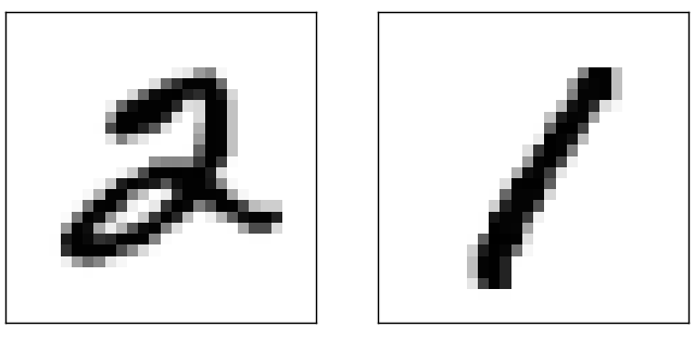
From this it follows that we can calculate the average darkness for each digit from 0 to 9. When receiving a new image, we calculate its darkness, and we guess that it shows a figure with the nearest average darkness. This is a simple procedure that is easy to program, so I will not write code — if it is interesting, it lies on GitHub . But this is already a serious improvement compared to random guesses - the code correctly recognizes 2,225 out of 10,000 images, that is, it gives an accuracy of 22.25%.

It is easy to find other ideas that achieve accuracy in the range from 20 to 50%. After working a little more, you can exceed 50%. But in order to achieve much greater accuracy, it is better to use authoritative MO algorithms. Let's try one of the most well-known algorithms, support vector machine or SVM. If you are unfamiliar with SVM, do not worry, we do not need to understand these details. We simply use the python library called scikit-learn, which provides a simple interface to the fast C library for SVM, known as LIBSVM .

If we run the sckit-learn SVM classifier on the default settings, we will get the correct classification 9,435 out of 10,000 (the code is available at the link). This is a great improvement compared to the naive approach of classifying images by darkness. This means that SVM works about as well as our NA, only a bit worse. In the following chapters, we will get acquainted with new techniques that will allow us to improve our NA so much that they overtake SVM.

But that's not all.The result of 9,435 out of 10,000 from scikit-learn is specified for the default settings. SVM has many parameters that can be adjusted, and you can look for parameters that improve this result. I will not go into details, they can be read in the article by Andreas Muller. He showed that having done the work on parameter optimization, it is possible to achieve an accuracy of at least 98.5%. In other words, a well-tuned SVM is mistaken only in one digit out of 70. A good result! Can NA achieve more?

It turns out they can. Today, a well-tuned NA overtakes any other known technology in the MNIST solution, including SVM. Record for 2013correctly classified 9,979 out of 10,000 images. And most of the technology used for this we will see in this book. This level of accuracy is close to human, and, perhaps, exceeds it, because several images from MNIST are difficult to decipher even to a person, for example:



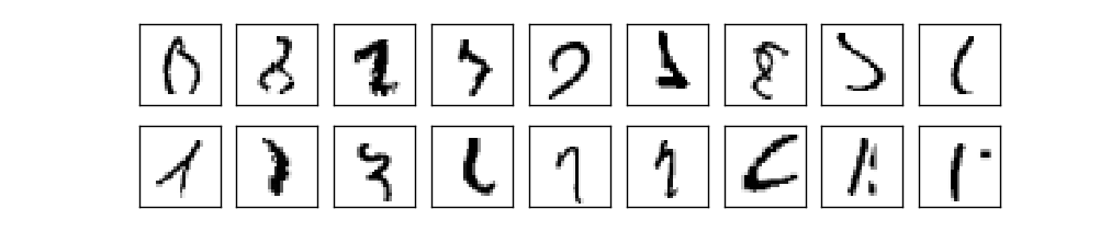
I think you will agree that they are difficult to classify! With such images in the MNIST dataset, it is surprising that the NN can correctly recognize all the images from 10,000, except 21. Programmers usually think that a complex algorithm is required to solve such a complex task. But even the National Assembly in the work-recordmans use fairly simple algorithms, which are small variations of those we discussed in this chapter. All complexity automatically appears during training based on training data. In a sense, the moral of our results and those contained in more complex works is that for some tasks

complex algorithm ≤ simple learning algorithm + good learning data

To deep learning

Although our network demonstrates impressive performance, it is achieved in a mysterious way. Weights and mixing nets are automatically detected. So, we have no ready explanation for how the network does what it does. Is it possible to find some way to understand the basic principles of classification by handwritten numbers? And is it possible, given them, to improve the result?

Let us reformulate these questions more rigidly: let us assume that in a few decades the National Assembly will turn into artificial intelligence (AI). Will we understand how this AI works? We may not understand the networks for us, with their weights and offsets, as they are automatically assigned. In the early years of AI research, people hoped that attempts at creating AI could also help us understand the principles underlying intelligence, and maybe even the workings of the human brain. However, in the end, it may turn out that we will not understand either the brain or the way AI works!

To deal with these questions, let us recall the interpretation of artificial neurons that I gave at the beginning of the chapter - that this is a way to weigh evidence. Suppose we want to determine if there is a person’s face in the image:







This problem can be approached in the same way as handwriting recognition: using image pixels as input for the NA, and at the output of the NA there will be one neuron that says, “Yes, this face”, or “No, this is not a face ".

Suppose we do this, but not using the learning algorithm. We will try to manually create a network by choosing the appropriate weights and offsets. How can we approach this? Forgetting the NA for a minute, we could break the task down into subtasks: does the image of the eyes have in the upper left corner? Is there an eye in the upper right corner? Is there a nose in the middle? Is there a mouth down in the middle? Do you have hair at the top? And so on.

If the answers to several of these questions are positive, or even “probably yes”, then we conclude that there may be a face in the image. Conversely, if the answers are negative, then the person is probably not.

This, of course, is an approximate heuristic, and it has many shortcomings. Perhaps this is a bald man, and he has no hair. Perhaps we can see only part of the face, or face at an angle, so that some parts of the face are closed. And yet, heuristics say that if we can solve subtasks using neural networks, then perhaps we can create an NA for face recognition, combining networks for subtasks. The following is a possible architecture of such a network, in which rectangles indicate subnets. This is not a realistic approach to solving the problem of face recognition: it is needed to help us intuitively understand the work of neural networks.


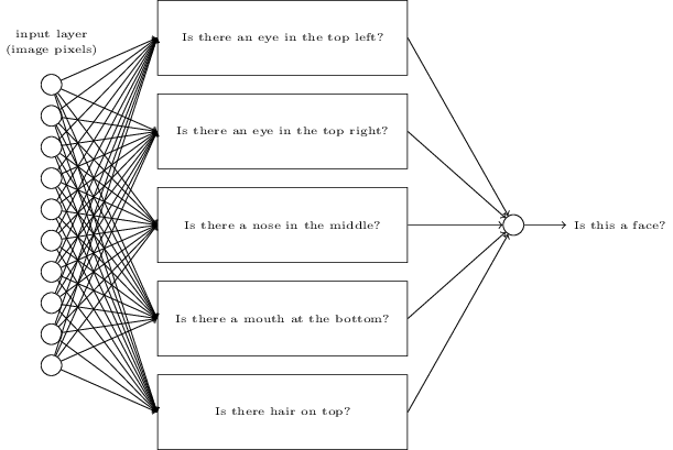
In the rectangles - subtasks: does the image of the eyes in the upper left corner? Is there an eye in the upper right corner? Is there a nose in the middle? Is there a mouth down in the middle? Do you have hair at the top? And so on.

It is possible that subnets can also be disassembled into components. Take the question of having an eye in the upper left corner. It can be disassembled into questions like: “Is there an eyebrow?”, “Are there eyelashes?”, “Is there a pupil?” And so on. Of course, the questions should contain information about the location - “Is the eyebrow located at the top left above the pupil?”, And so on - but let's simplify it for now. Therefore, the network that answers the question about the presence of an eye can be disassembled into components:


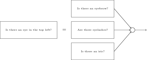
“Is there an eyebrow?”, “Are there eyelashes?”, “Is there a pupil?”

These questions can be further divided into small ones, step by step through many layers. As a result, we will work with subnets that answer such simple questions that they can be easily disassembled at the pixel level. These questions may concern, for example, the presence or absence of the simplest forms in certain places of the image. Individual neurons associated with pixels will be able to respond to them.

The result will be a network that breaks down very difficult questions - the presence of a face on the image - to very simple questions that can be answered at the level of individual pixels. It will do this through a sequence of many layers in which the first layers answer very simple and concrete questions about the image, and the latter create a hierarchy of more complex and abstract concepts. Networks with such a multi-layered structure — two or more hidden layers — are called deep neural networks (GNS).

Of course, I didn’t talk about how to do this recursive subnetting. It is definitely impractical to manually pick weights and offsets. We would like to use training algorithms so that the network automatically learns weights and offsets - and through them hierarchies of concepts - based on training data. Researchers in the 1980s and 1990s tried to use stochastic gradient descent and backward propagation to train the STS. Unfortunately, with the exception of a few special architectures, they did not succeed. The networks were trained, but very slowly, and in practice it was too slow for it to be used in any way.

Since 2006, several technologies have been developed that allow teaching STS. They are based on stochastic gradient descent and back propagation, but contain new ideas. They allowed to train much deeper networks - today people quietly train networks with 5-10 layers. And it turns out that they solve many problems much better than shallow NAs, that is, networks with one hidden layer. The reason, of course, is that the STS can create a complex hierarchy of concepts. This is similar to how programming languages ​​use modular schemes and ideas of abstractions so that they can create complex computer programs. Comparing a deep NA with a shallow NA is about how to compare a programming language that can make function calls to a language that does not. Abstraction in the NA looks not like in programming languages,but is of the same importance.