Logistics shares for the collection of recyclables

Instead of intro

When the processes of waste collection and recycling will be fully developed in Russia, it is not easy to say, but I want to avoid participating in landfill replenishment now. Therefore, in many large cities, one way or another, there are volunteer movements that are engaged, in particular, in separate collection.

In Novosibirsk, such an activity is formed around the Green Squirrel action, in which once a month, ecologically concerned citizens bring accumulated recycled household waste to predetermined places at a certain time. By the same time, a rented truck arrives there, which transports the collected and sorted salvage to the site, from where it is redistributed between various processing enterprises. The action has existed since 2014, and since that time the number of recycling points has increased significantly, as well as its volumes. For routing the trucks, the gaze alone was lacking, and we began to develop optimization models to minimize transportation costs. This article is the first of these models.

In Section 1, I will describe in detail and with illustrations the scheme for organizing the action. Further, in section 2, the problem of minimizing transportation costs will be formalized as a routing problem for heterogeneous vehicles with time windows (heterogenious fleet vehicle routing problem with time windows). Section 3 is devoted to solving this problem using a freely distributed package for solving mixed-integer linear problems of mathematical programming GLPK.

1. Action "Green Squirrel"

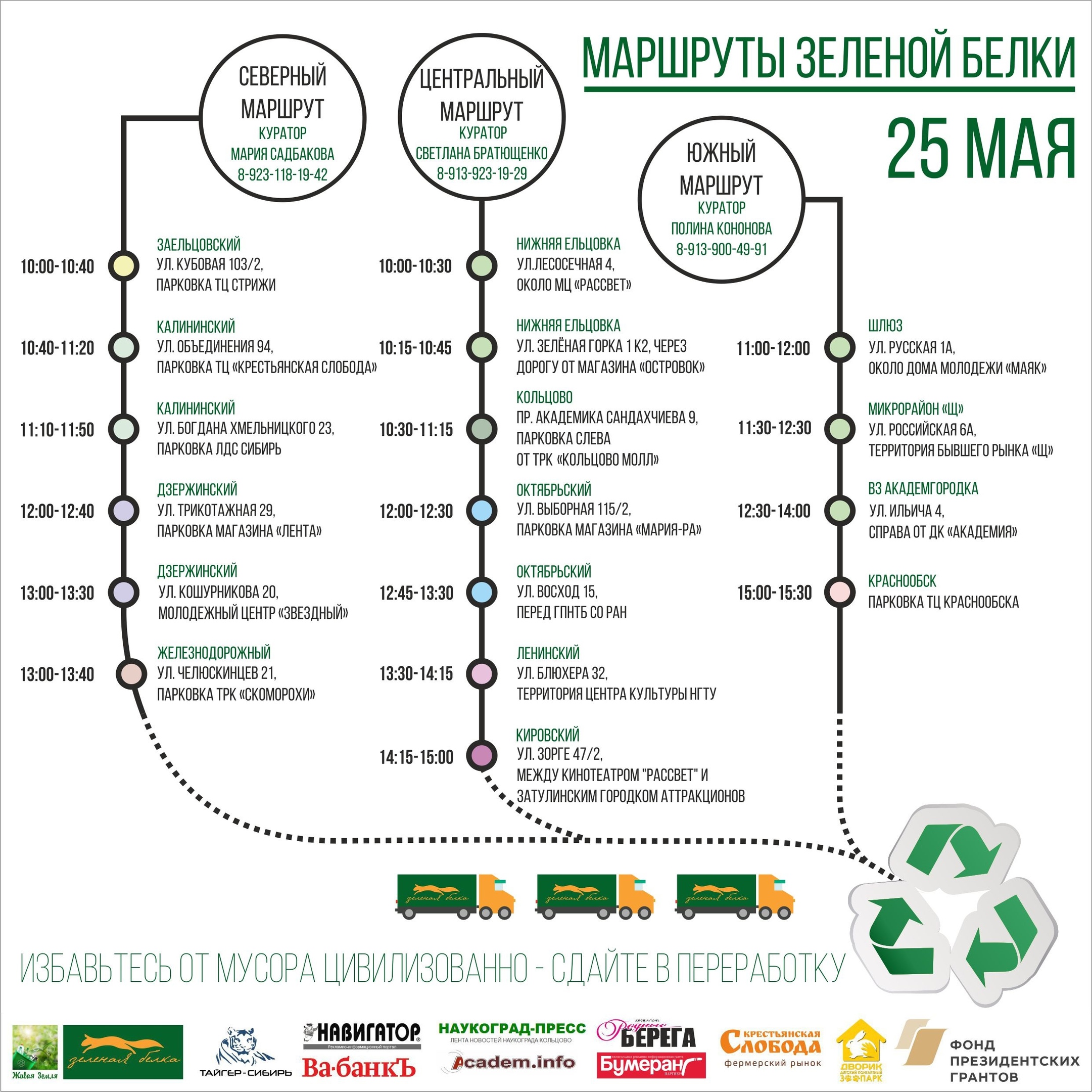
Beginning in 2014, the Live Earth initiative group has been conducting a monthly campaign on separate collection of recycled Green Squirrel in Novosibirsk. At the time of writing the article for recycling with a number of reservations accepted plastic waste labeled PET, PE, PP, PS, glass, aluminum, iron, household appliances, waste paper and more. More than 50 volunteers participate in the preparation and holding of the action. The promotion is not commercial, participation in it is free and does not imply a monetary reward.
')
Points

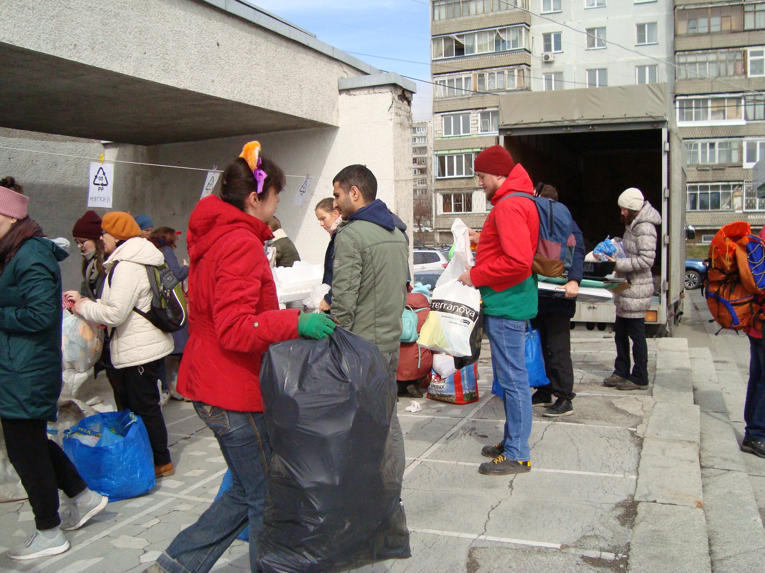
The action is held in 17 points of the city, spaced from each other at distances covered by the car during the time from 15 to 90 minutes. In the photo one of these points: on the left along the wall there are bags for collecting various plastic fractions, on the right is a truck into which everything is loaded later, and in the center is a volunteer with ears.

The curators, who have time limits in which they are ready to perform their duties, organize all the activity at the point. When planning the action, the curators report the time interval within which the action must take place at their point.

There is also data on average volumes of recycled materials collected at each of the points.

Routes

Points are organized into routes, sequentially driven by truck. Truck movements are monitored by route curators who monitor the operational situation and make decisions on handling special events.

Trucks

They are rented out on a general basis as part of proposals for the hourly rental of freight transport. It is not possible to compact plastic in place, therefore the main parameter characterizing the truck is the volume of the body. Load capacity in our case is not a limiting factor.

The main expenses of the action are connected precisely with the payment of the rental of trucks, so its reduction is crucial for the existence and development of our action, which acquires institutional significance in the sense of forming ideas about responsible consumption. Next will be described an approach to solving this issue, based on the use of discrete optimization methods, namely mathematical programming.

2. Formalization

When constructing a mathematical model, we will remain within the framework of linear mixed-integer programs, for understanding of which knowledge of class 7 algebra is sufficient.

The only difficulty can be associated with the use of abstract symbols and summation signs in formulas. I hope this does not scare readers who have infrequent meetings with mathematical texts.

The optimization model can be divided into four components:

the formation of groups of points that make up a separate route;
determination of the detour pattern of each group;
meeting the requirements for the time of arrival of the truck at each of the points;
determining the type of truck needed to service each of the routes.

Consider each of the parts, introducing as necessary the necessary notation.

Formation of groups of points

Let be

V = \ {1, \ dots, n \}

$V = \ {1, \ dots, n \}$ there is a set of indices of collection points for recyclables, and the site where the collected recyclables are then transported - we will call it a depot - has an index of 0. We set

\ bar {V} = V \ cup \ {0 \}

$\ bar {V} = V \ cup \ {0 \}$

Each group of points forms a separate route. Through

R

$R$ denote a set of route numbers.

Let the value

z_{i r}, i i n I, r i n R

$z_ {ir}, i \ in I, r \ in R$ equals one if point

i

$i$ included in the route with the number

r

$r$ and zero otherwise. Then the requirement that the point

i i n V

$i \ in V$ must enter one of the routes can be written by equality

s u m_{r i n R} z_{i r} = z_{i 1} + z_{i 2} + d o t s + z_{i n} = 1.

$\ sum_ {r \ in R} z_ {ir} = z_ {i1} + z_ {i2} + \ dots + z_ {in} = 1.$

Depot must enter all routes:

z_{0 r} = 1, r i n R

$z_ {0r} = 1, r \ in R$

Subtleties

Unfortunately, such a recording creates computational problems related to the symmetry of an admissible region. It can be eliminated by adding a number of restrictions that ensure the choice of a lexicographically minimal partition. More in Russian about this can be read, for example, here .

1 - z_{i r} l e q s u m_{j = 1}^{i - 1} l e f t (1 - s u m_{k = 1}^{r - 1} z_{j k} r i g h t) + s u m_{k = 1}^{r - 1} z_{i k}, q u a d i i n I, r i n R, r l e q i .

$1-z_ {ir} \ leq \ sum_ {j = 1} ^ {i-1} \ left (1- \ sum_ {k = 1} ^ {r-1} z_ {jk} \ right) + \ sum_ { k = 1} ^ {r-1} z_ {ik}, \ quad i \ in I, r \ in R, r \ leq i.$

Determination of the detour pattern

Routes are an alternating sequence of points and crossings between them. Formally, they all start at one of the points of the set

V

$V$ and end at the depot, but it will be easier to assume that all routes are cyclical. This assumption does not change the essence, but makes all the peaks the same: in this case there are no end peaks, they are all transit peaks.

For points

i, j i n b a r V

$i, j \ in \ bar {V}$ and route

r i n R

$r \ in R$ let's get the variable

x_{i j r}

$x_ {ijr}$ equal to one if the route c number

r

$r$ the truck makes the move from the point

i

$i$ exactly

j

$j$ and zero otherwise.

Then we demand, firstly, that the truck moving on the route

r i n R

$r \ in R$ visited point

i i n V

$i \ in V$ if, after dividing it into groups, it fell into the group with the number

r

$r$ :

s u m_{j i n b a r V} x_{j i r} = z_{i r}, q u a d i i n b a r V, r i n R .

$\ sum_ {j \ in \ bar {V}} x_ {jir} = z_ {ir}, \ quad i \ in \ bar {V}, r \ in R.$

Secondly, the truck after arriving at the point

i i n b a r V

$i \ in \ bar {V}$ must go with her.

s u m_{j i n b a r V} x_{j i r} = s u m_{j i n b a r V} x_{i j r}, q u a d i i n b a r V, r i n R .

$\ sum_ {j \ in \ bar {V}} x_ {jir} = \ sum_ {j \ in \ bar {V}} x_ {ijr}, \ quad i \ in \ bar {V}, r \ in R .$

You may notice that these limits allow values

x_{i j r}

$x_ {ijr}$ set routes, which are a set of non-intersecting loops. Routes of this type, of course, do not make sense, and you want to add a number of restrictions to avoid this.

About elimination of subcycles

One way would be to introduce auxiliary non-negative values.

f_{i j r}, i, j i n b a r V, r i n R

$f_ {ijr}, i, j \ in \ bar {V}, r \ in R$ Recorded using these values, the set of relations eliminates combinations of values.

x_{i j r}

$x_ {ijr}$ that specify routes that are not connected loop.

s u m_{i i n V} f_{0 j r} = s u m_{i i n V} z_{i r}, q u a d r i n R,

$\ sum_ {i \ in V} f_ {0jr} = \ sum_ {i \ in V} z_ {ir}, \ quad r \ in R,$

f_{i j r} l e q n x_{i j r}, q u a d i i n b a r V, j i n b a r V, r i n R,

$f_ {ijr} \ leq nx_ {ijr}, \ quad i \ in \ bar {V}, j \ in \ bar {V}, r \ in R,$

s u m_{j i n b a r V} f_{j i r} = s u m_{j i n b a r V} f_{i j r} + z_{i r}, q u a d i i n V, r i n R .

$\ sum_ {j \ in \ bar {V}} f_ {jir} = \ sum_ {j \ in \ bar {V}} f_ {ijr} + z_ {ir}, \ quad i \ in V, r \ in R.$

These ratios set the flow from the depot to the rest of the route points. At each intermediate point, a unit of flow is absorbed, so in order for a network to have a power flow equal to the number of points minus one, it is necessary that the route be connected.

Satisfying requirements at the time of arrival of the truck at each of the points

In other words, it is necessary to visit points only inside the time windows indicated by the curators. Through

B_{i}

$B_i$ and

E_{i}

$E_i$ denote, respectively, the beginning and end of the time interval in which the curator of the point

i

$i$ may attend her.

To track the implementation of these restrictions, we will need information about the time spent by the truck during stops and crossings on the route. Through

L_{i}, i i n V

$L_i, i \ in V$ denote the duration of loading at the point

i

$i$ and through

D_{i j}, i, j i n b a r V

$D_ {ij}, i, j \ in \ bar {V}$ - time of moving from point

i

$i$ exactly

j

$j$ Make a reservation that

D_{0 i} = 0

$D_ {0i} = 0$ for all

i i n b a r V

$i \ in \ bar {V}$ , and generally can be performed

D_{i j} n e q D_{j i}

$D_ {ij} \ neq D_ {ji}$ for any

i n e q j

$i \ neq j$

We introduce variable non-negative values

a_{i}, i i n b a r V

$a_i, i \ in \ bar {V}$ and

w_{i r}, i i n b a r V, r i n R

$w_ {ir}, i \ in \ bar {V}, r \ in R$ equal to arrival and waiting times

i

$i$ when driving on the route

r

$r$ , respectively. For the entered values, the following relationships should be fulfilled.

Waiting time can not be less than the time required for loading

w_{i r} g e q L_{i} z_{i r}, q u a d i i n b a r V, r i n R,

$w_ {ir} \ geq L_iz_ {ir}, \ quad i \ in \ bar {V}, r \ in R,$

and is zero if the point does not belong to the route

r

$r$

w_{i r} l e q M z_{i r}, q u a d i i n b a r V, r i n R,

$w_ {ir} \ leq Mz_ {ir}, \ quad i \ in \ bar {V}, r \ in R,$

Time of arrival at the point

j

$j$ calculated through the corresponding times for the preceding point

i

$i$ There is a fairly large constant

M

$M$ is used to eliminate unnecessary dependencies when moving between

i

$i$ and

j

$j$ not done

a_{i} + s u m_{r i n R} w_{i r} + D_{i j} l e q a_{j} + M (1 - s u m_{r i n R} x_{i j r}), q u a d i i n I, j i n V,

$a_i + \ sum_ {r \ in R} w_ {ir} + D_ {ij} \ leq a_j + M (1 - \ sum_ {r \ in R} x_ {ijr}), \ quad i \ in I, j \ in V,$

Arrival and departure of the truck must be within the designated interval curator.

a_{i} g e q B_{i}, q u a d i i n V,

$a_i \ geq B_i, \ quad i \ in V,$

a_{i} + s u m_{r i n R} w_{i r} l e q E_{i}, q u a d i i n V .

$a_i + \ sum_ {r \ in R} w_ {ir} \ leq E_i, \ quad i \ in V.$

Determining the type of truck needed to service each of the routes
Denote the many types of trucks that are available for rent through

T

$T$ Truck type

t i n T

$t \ in T$ characterized by body volume

C_{t}

$C_t$ and the cost of hourly rent

P_{t}

$P_t$ Minimum truck rental type

t

$t$ denote by

U_{t}^{0}

$U_t ^ 0$ Recycled volume collected at point

i i n V

$i \ in V$ denote by

G_{i}

$G_i$

We introduce variables

y_{t r}, t i n T, r i n R

$y_ {tr}, t \ in T, r \ in R$ equal to one if truck type

t

$t$ assigned to service route with number

r

$r$ and zero otherwise.

Integer variables

u_{t r}, t i n T, r i n R

$u_ {tr}, t \ in T, r \ in R$ set the time of renting a truck type

t

$t$ serving route number

r

$r$
For each route,

r i n R

$r \ in R$ , you must assign the type of truck:

s u m_{t i n T} y_{t r} = 1, q u a d r i n R

$\ sum_ {t \ in T} y_ {tr} = 1, \ quad r \ in R$

In accordance with the splitting of points between routes, some routes may be trivial, that is, contain only depot. If route

r

$r$ nontrivial, the truck assigned to it is rented for at least

U_{t}^{0}

$U_t ^ 0$ hours

u_{t r} g e q U_{t}^{0} (y_{t r} - s u m_{i i n V} z_{i r}), q u a d t i n T, r i n R .

$u_ {tr} \ geq U_t ^ 0 (y_ {tr} - \ sum_ {i \ in V} z_ {ir}), \ quad t \ in T, r \ in R.$

At the same time, the duration of the lease should also exceed the total duration of stops and crossings in the route.

u_{t r} g e q s u m_{i i n V} s u m_{j i n b a r V} D_{i j} x_{i j r} + s u m_{i i n b a r V} w_{i r} - M (1 - y_{t r}), q u a d r i n R, t i n T .

$u_ {tr} \ geq \ sum_ {i \ in V} \ sum_ {j \ in \ bar {V}} D_ {ij} x_ {ijr} + \ sum_ {i \ in \ bar {V}} w_ { ir} -M (1-y_ {tr}), \ quad r \ in R, t \ in T.$

Add constraints providing the property: if a truck is of type

t

$t$ not assigned to route

r

$r$ , its rental time is zero.

u_{t r} l e q M y_{t r} .

$u_ {tr} \ leq My_ {tr}.$

All recyclables collected at the points of the route should fit in the back of the truck.

s u m_{i i n V} G_{i} z_{i r} l e q s u m_{t i n T} C_{t} y_{t r}, q u a d r i n R .

$\ sum_ {i \ in V} G_iz_ {ir} \ leq \ sum_ {t \ in T} C_ty_ {tr}, \ quad r \ in R.$

Finally, our goal is to minimize the cost of renting a truck, which, using the entered notation, is written as

s u m_{t i n T} s u m_{r i n R} P_{t} u_{t r}

$\ sum_ {t \ in T} \ sum_ {r \ in R} P_tu_ {tr}$

Search for a solution

It is easy to make sure that all the expressions involved in the optimization model are linear functions of variables, therefore, to find accurate and approximate solutions, you can use standard packages for solving problems of mixed-integer programming such as Gurobi , CPLEX , Xpress , ORtools , SCIP , BLIS , etc.
We write the model of minimizing transportation costs in the GMPL language. This will allow us to use the freely distributed GLPK package for our purposes. For writing code and debugging the model, it will be convenient to download the GUSEK development environment , which already contains GLPK in its composition.

GUSEK looks like this:

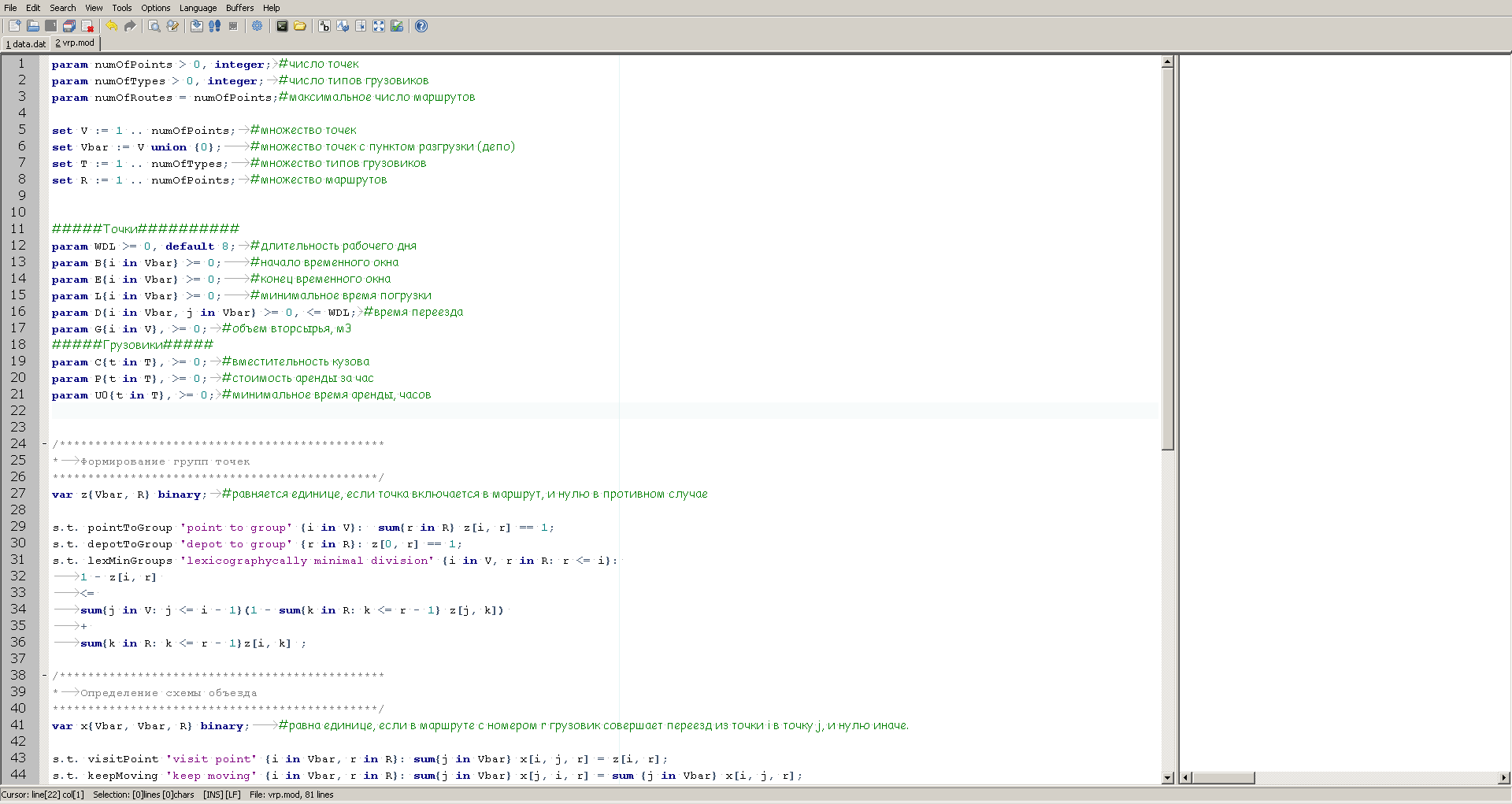
On the left, we see a description of the model, and on the right, a window displaying information about the progress of the calculations that the solver will deliver after launch.

Full description of the model

param numOfPoints > 0, integer; #  param numOfTypes > 0, integer; #   param numOfRoutes = numOfPoints;#   set V := 1 .. numOfPoints; #  set Vbar := V union {0}; #     () set T := 1 .. numOfTypes; #   set R := 1 .. numOfPoints; #  ############### param WDL >= 0, default 8; #   param B{i in Vbar} >= 0; #   param E{i in Vbar} >= 0; #   param L{i in Vbar} >= 0; #   param D{i in Vbar, j in Vbar} >= 0, <= WDL; #  param G{i in V}, >= 0; # , 3 ########## param C{t in T}, >= 0; #  param P{t in T}, >= 0; #    param U0{t in T}, >= 0; #  ,  /********************************************** *    **********************************************/ var z{Vbar, R} binary; # ,     ,      st pointToGroup 'point to group' {i in V}: sum{r in R} z[i, r] == 1; st depotToGroup 'depot to group' {r in R}: z[0, r] == 1; st lexMinGroups 'lexicographycally minimal division' {i in V, r in R: r <= i}: 1 - z[i, r] <= sum{j in V: j <= i - 1}(1 - sum{k in R: k <= r - 1} z[j, k]) + sum{k in R: k <= r - 1}z[i, k] ; /********************************************** *    **********************************************/ var x{Vbar, Vbar, R} binary; # ,    c  r      i   j,   . st visitPoint 'visit point' {i in Vbar, r in R}: sum{j in Vbar} x[i, j, r] = z[i, r]; st keepMoving 'keep moving' {i in Vbar, r in R}: sum{j in Vbar} x[j, i, r] = sum {j in Vbar} x[i, j, r]; var f{Vbar, Vbar, R} >= 0; #,  . st flowFromDepot 'flow from depot' {r in R}: sum{i in V} f[0, i, r] == sum{i in V} z[i, r]; st flowAlongActiveArcs 'flow along active arcs' {i in Vbar, j in Vbar, r in R}: f[i, j, r] <= numOfPoints * x[i, j, r]; st flowConservation 'flow conservation' {i in V, r in R}: sum{j in Vbar} f[j, i, r] == sum{j in Vbar} f[i, j, r] + z[i, r]; var a{i in V} >= 0; #     var w{i in Vbar, r in R} >= 0; #     st wait 'wait'{i in Vbar, r in R}: w[i, r] >= L[i] * z[i, r]; st dontWait 'dont wait'{i in Vbar, r in R}: w[i, r] <= (E[i] - B[i]) * z[i, r]; st arrivalTime 'arrival time' {i in V, j in V}: a[i] + sum{r in R}w[i, r] + D[i,j] <= a[j] + 3 * WDL * (1 - sum{r in R} x[i, j, r]); st arriveAfter 'arrive after' {i in V}: a[i] >= B[i]; st departBefore 'depart before' {i in V}: a[i] + sum{r in R}w[i, r] <= E[i]; /********************************************** *   ,       **********************************************/ var y{t in T, r in R}, binary; # ,    t       r,   . var u{t in T, r in R}, integer, >= 0; #    t,     rst assignVehicle 'assign vehicle' {r in R}: sum{t in T} y[t,r] == 1; st rentTime 'rent time' {r in R, t in T}: u[t, r] >= sum{i in V, j in Vbar}D[i, j] * x[i, j, r] + sum{i in Vbar}w[i, r] - WDL * (1 - y[t, r]); st minRentTime 'minimal rent time' {r in R, t in T}: u[t, r] >= U0[t] * (y[t, r] - sum{i in V}z[i, r]); st noRent 'no rent' {t in T, r in R}: u[t, r] <= WDL * y[t, r]; st fitCapacity 'fit capacity' {r in R}: sum{i in V} G[i] * z[i, r] <= sum{t in T} C[t] * y[t, r]; minimize rentCost: sum{t in T, r in R} P[t] * u[t, r]; solve; /********************************************** *     **********************************************/ printf{i in V, r in R} (if 0.1 < z[i,r] then "point %s to group %s\n" else ""), i, r, z[i,r]; printf{r in R, i in Vbar, j in Vbar} (if 0.1 < x[i, j, r] then "route %s: %s -> %s\n" else ""), r, i, j; printf{i in V} "point %s arrive between %s and %s (actual = %s)\n", i, B[i], E[i], a[i]; end;

For a quick start, I also add data prepared for use in the model, taken from the head:

Input data

 data; param numOfPoints := 9; #  param numOfTypes := 6; #   ############### param : B E L := 0 0 8 1 1 0 8 1 2 0 8 1 3 0 8 1 4 0 8 1 5 0 8 1 6 0 8 1 7 0 8 1 8 0 8 1 9 0 8 1; param D default 0 : 0 1 2 3 4 5 6 7 8 9 := 0 . . . . . . . . . . 1 0.1 0.3 0.2 0.1 0.2 0.1 0.2 0.1 0.2 0.1 2 0.3 0.2 0.2 0.1 0.2 0.1 0.2 0.1 0.2 0.1 3 0.4 0.3 0.2 0.1 0.2 0.1 0.2 0.1 0.2 0.1 4 0.4 0.4 0.2 0.1 0.2 0.1 0.2 0.1 0.2 0.1 5 0.1 0.2 0.2 0.1 0.2 0.1 0.2 0.1 0.2 0.1 6 0.5 0.5 0.2 0.1 0.2 0.1 0.2 0.1 0.2 0.1 7 0.3 0.2 0.2 0.1 0.2 0.1 0.2 0.1 0.2 0.1 8 0.2 0.1 0.2 0.1 0.2 0.1 0.2 0.1 0.2 0.1 9 0.5 0.2 0.2 0.1 0.2 0.1 0.2 0.1 0.2 0.1; param G := 1 1 2 2 3 1 4 2 5 1 6 2 7 1 8 2 9 1; ########## param : C P := 1 8 500 2 10 500 3 14 600 4 18 650 5 25 700 6 35 800; param U0 default 2; #  ,  end;

After copying the model code into a file with the name, for example, model.mod, and the input data is in the data.dat file, everything is ready for launch. Set a limit on the calculation time of 100 seconds (this is done using the –tmlim key [time in seconds]), passing the path to the file with input data (using the –d key [file path]),

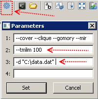
and hit F5. If successful, messages will appear in the window on the right, and after a hundred seconds we will have the best solution in our hands, which GLPK managed to find in the allotted time.

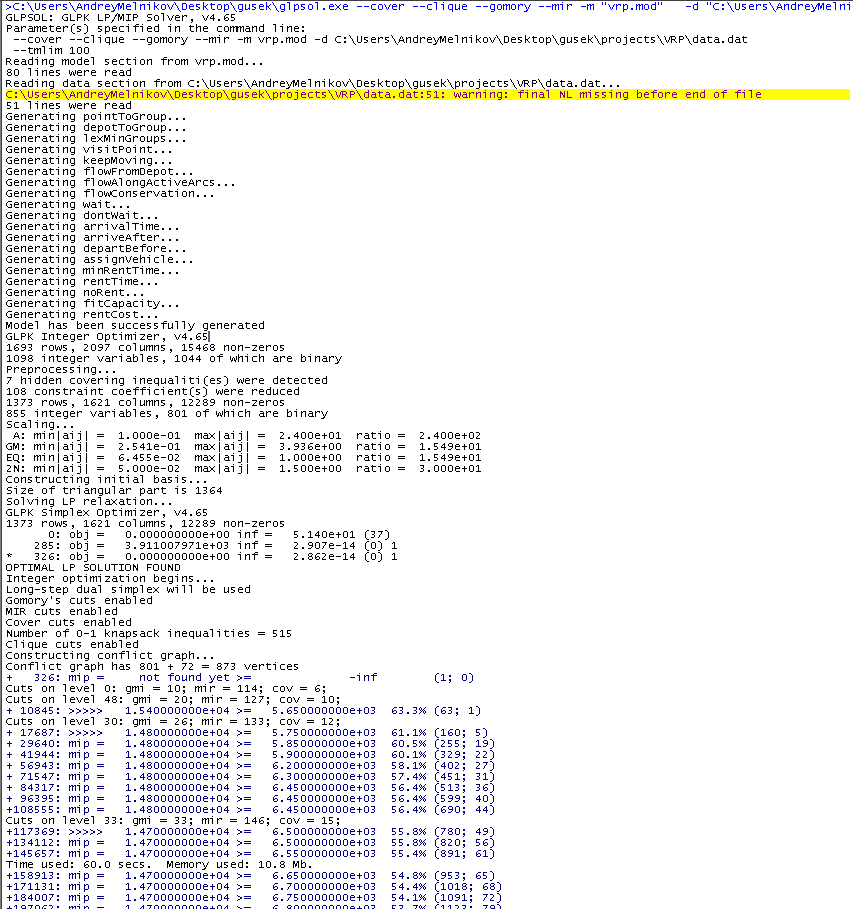
In the blue text, we are interested in the value after the caption "mip =". As you can see, it decreases from time to time. In the process, there are all new solutions, the value of transportation costs for the best of which is displayed in this column (so far there are 14,700). The next number is a lower bound for the best existing one, i.e. the optimal solution. Initially, the assessment is significantly underestimated, but over time is refined, that is, increases. The values on the left and on the right come closer, and the relative gap between them at the time of the screenshot is 54.1%. As soon as this number becomes zero, the algorithm will prove that the best solution found is the best possible. To wait for this event in practice is not always justified, and not only because it takes a long time, but it is important to make a reservation that, as a rule, a good solution is found relatively quickly, and the main time costs are related to the refinement of the estimate required for proof of non-improvement.

Instead of conclusion

The routing tasks are extremely difficult computationally, and with the increase in the number of points that need to be visited, the time required for the solver to find a solution and prove its optimality grows rapidly. However, for fairly small examples, the solver can build a good set of routes in a reasonable time and can be used to support decision making. An analysis of the proposed routing options has helped us discover significant opportunities to reduce costs, and this is crucial for the existence and development of the promotion.

Our further efforts were directed towards working with uncertainty in the volumes of recycled materials collected at the points. We are developing a range of stochastic programming models for making strategic and operational decisions in truck routing. If the topic turns out to be relevant and arouses interest, I will write about it too, because soon we all will have to immerse ourselves in environmental issues much more thoroughly, in which I wish us success.

Source: https://habr.com/ru/post/456310/

All Articles