Distributed computing in Julia

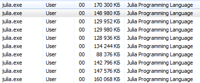
If the previous article was more likely to be a starter, then now is the time to test Julia’s ability to parallelize on her machine.
Multicore or distributed processing
The implementation of parallel computing with distributed memory is provided by the Distributed module as part of the standard library supplied with Julia. Most modern computers have more than one processor, and several computers can be combined into a cluster. Using the power of these multiple processors allows you to perform many calculations faster. The performance is influenced by two main factors: the speed of the processors themselves and the speed of their access to the memory. In a cluster, it is clear that this CPU will have the fastest access to RAM on the same computer (node). Perhaps even more surprisingly, such problems are relevant to a typical multi-core laptop due to differences in the speed of the main memory and cache. Therefore, a good multiprocessor environment should allow controlling the “ownership” of a part of the memory by a specific processor. Julia provides a multiprocessor, messaging-based environment that allows programs to run simultaneously on multiple processes in different memory domains.
The implementation of messaging in Julia is different from other media such as MPI [1] . Communication in Julia is usually “one-way”, which means that the programmer needs to explicitly control only one process in a two-process operation. In addition, these operations usually do not look like “sending a message” and “receiving a message”, but rather resemble higher-level operations, such as calls to user-defined functions.
Distributed programming in Julia is based on two primitives: remote links and remote calls . A remote reference is an object that can be used from any process to reference an object stored in a specific process. A remote call is a request from one process to call a specific function on certain arguments of another (possibly the same) process.
Remote links come in two forms: Future and RemoteChannel .
The remote call returns the Future and does it immediately; the process that made the call goes to its next operation, while the remote call is somewhere else. You can wait for the remote call to complete with the wait command for the returned Future , and you can also get the full value of the result using fetch .
On the other hand, we have RemoteChannels that are overwritten. For example, several processes can coordinate their processing by referring to the same remote channel. Each process has an associated id. The process that provides the Julia interactive prompt always has an identifier of 1. The processes used by default for parallel operations are called "employees." When there is only one process, process 1 is considered working. Otherwise, all processes other than process 1 are considered workers.

Let's get down to it. Startup with julia -pn provides n workflows on the local computer. It usually makes sense that n is equal to the number of CPU threads (logical cores) on a machine. Note that the -p argument implicitly loads the Distributed module.
For Linux users, actions with the console should not cause difficulties, t.ch. This educational program is intended for inexperienced users of Windows.
The terminal Julia (REPL) provides the ability to use the system commands:
julia> pwd() # "C:\\Users\\User\\AppData\\Local\\Julia-1.1.0" julia> cd("C:/Users/User/Desktop") # julia> run(`calc`) # # Windows. # Process(`calc`, ProcessExited(0)) using these commands, you can run Julia from Julia, but it's better not to get involved
It would be more correct to run cmd from julia / bin / and execute there the julia -p 2 command or an option for fans of starting from a shortcut: on the desktop, create a notepad document with such contents C:\Users\User\AppData\Local\Julia-1.1.0\bin\julia -p 4 (the address and the number of processes specify your own ) and save it as a text document with the name run.bat . Here, now you have a Julia system startup file for 4 cores on your desktop.
$ ./julia -p 2 julia> r = remotecall(rand, 2, 2, 2) Future(2, 1, 4, nothing) julia> s = @spawnat 2 1 .+ fetch(r) Future(2, 1, 5, nothing) julia> fetch(s) 2×2 Array{Float64,2}: 1.18526 1.50912 1.16296 1.60607 The first argument for remotecall is the function being called.
Most parallel programs in Julia do not refer to specific processes or the number of available processes, but the remote call is considered a low-level interface that provides more precise control.
The second argument for remotecall is the identifier of the process that will do the work, and the remaining arguments will be passed to the called function. As you can see, in the first row we asked process 2 to build a random 2 on 2 matrix, and in the second row we asked to add 1 to it. The result of both calculations is available in two futures, r and s. The spawnat macro evaluates the expression in the second argument of the process specified in the first argument. Sometimes you may need a remotely calculated value. This usually happens when you read from a remote object to get the data needed for the next local operation. For this there is a function remotecall_fetch . This is equivalent to fetch (remotecall (...)) , but more efficiently.
Remember that getindex(r, 1,1) equivalent to r[1,1] , so this call retrieves the first element of the future r .
The remotecall remote call remotecall not particularly convenient. The @spawn macro simplifies the work. It works with an expression, not a function, and chooses where to perform the operation for you:
julia> r = @spawn rand(2,2) Future(2, 1, 4, nothing) julia> s = @spawn 1 .+ fetch(r) Future(3, 1, 5, nothing) julia> fetch(s) 2×2 Array{Float64,2}: 1.38854 1.9098 1.20939 1.57158 Notice that we used 1 .+ Fetch(r) instead of 1 .+ r . This is because we do not know where the code will be executed, therefore, in general, a sample may be required to move r into the process that performs the addition. In this case, @spawn is smart enough to perform calculations for the process to which r belongs, so fetch will be non-operational (no work is done). (It is worth noting that spawn is not embedded, but is defined as a macro in Julia. You can define your own such constructs.)
It is important to remember that after retrieving, Future will cache its value locally. Further calls to fetch do not entail a network jump. After all the referenced futures are selected, the deleted stored value is deleted.
@async is similar to @spawn , but it runs tasks only in a local process. We use it to create a “filing” task for each process. Each task selects the next index to be calculated, then waits for the process to complete and repeats until we have run out of indexes.
Note that the feeder tasks do not begin to be executed until the main task reaches the end of the @sync block, after which it gives up control and waits for all local tasks to complete before returning from the function.
As for v0.7 and above, feeder tasks can share state via nextidx, because they all run in the same process. Even if tasks are scheduled together, in some contexts a lock may be required, for example, during asynchronous I / O. This means that context switching occurs only at well-defined points: in this case, when remotecall_fetch is remotecall_fetch . This is the current state of the implementation, and it may change in future versions of Julia, as it is designed so that you can perform up to N tasks in M processes, or M: N Threading . Then a nextidx lock acquisition / release model is nextidx , since it is not safe to allow several processes to read and write resources at the same time.
Your code must be available to any process that runs it. For example, enter the following in the Julia command line:
julia> function rand2(dims...) return 2*rand(dims...) end julia> rand2(2,2) 2×2 Array{Float64,2}: 0.153756 0.368514 1.15119 0.918912 julia> fetch(@spawn rand2(2,2)) ERROR: RemoteException(2, CapturedException(UndefVarError(Symbol("#rand2")) Stacktrace: [...] Process 1 was aware of the rand2 function, but process 2 was not. Most often, you will download code from files or packages, and you will have considerable flexibility in controlling which processes load code. Consider the DummyModule.jl file containing the following code:
module DummyModule export MyType, f mutable struct MyType a::Int end f(x) = x^2+1 println("loaded") end To reference MyType in all processes, DummyModule.jl must be loaded in each process. A call to include ('DummyModule.jl') loads it for only one process. To load it into each process, use the @everywhere macro (run Julia with the command julia -p 2):
julia> @everywhere include("DummyModule.jl") loaded From worker 3: loaded From worker 2: loaded As usual, this does not make the DummyModule available to any process that requires use or import. Moreover, when a DummyModule is included in the scope of one process, it is not included in any other:
julia> using .DummyModule julia> MyType(7) MyType(7) julia> fetch(@spawnat 2 MyType(7)) ERROR: On worker 2: UndefVarError: MyType not defined ⋮ julia> fetch(@spawnat 2 DummyModule.MyType(7)) MyType(7) However, it is still possible, for example, to send MyType to the process that loaded the DummyModule, even if it is not in scope:
julia> put!(RemoteChannel(2), MyType(7)) RemoteChannel{Channel{Any}}(2, 1, 13) The file can also be preloaded in several processes at startup with the -L flag, and the driver script can be used to control the calculations:
julia -p <n> -L file1.jl -L file2.jl driver.jl The Julia process that executes the driver script in the example above has an id of 1, just like the process that provides the interactive prompt. Finally, if DummyModule.jl is not a separate file, but a package, then using DummyModule will load DummyModule.jl in all processes, but only transfer it to the scope of the process for which the usage was caused.
Running and managing workflows
The basic installation of Julia has built-in support for two types of clusters:
- The local cluster specified with the -p option, as shown above.
- Cluster machines using the --machine-file option. It uses the ssh login without a password to start Julia workflows (along the same path as the current host) on the specified machines.

The functions addprocs , rmprocs , worker, and others are available as software tools for adding, deleting, and querying processes in a cluster.
julia> using Distributed julia> addprocs(2) 2-element Array{Int64,1}: 2 3 The Distributed module must be explicitly loaded into the main process before calling addprocs . It automatically becomes available for workflows. Note that workers do not run the startup script ~/.julia/config/startup.jl and they do not synchronize their global state (such as global variables, definitions of new methods and loaded modules) with any of the other running processes. Other types of clusters can be supported by writing your own ClusterManager , as described below in the ClusterManager section.
Actions with data
Sending messages and moving data make up the bulk of the overhead in a distributed program. Reducing the number of messages and the amount of data sent is critical to achieving performance and scalability. For this, it is important to understand the movement of data performed by various designs of Julia’s distributed programming.
fetch can be considered as an explicit operation of moving data, since it directly requests the movement of an object to the local machine. @spawn (and several related constructs) also moves data, but this is not so obvious, so this can be called an implicit data movement operation. Consider these two approaches to constructing and squaring a random matrix:
Way times:
julia> A = rand(1000,1000); julia> Bref = @spawn A^2; [...] julia> fetch(Bref); Method two:
julia> Bref = @spawn rand(1000,1000)^2; [...] julia> fetch(Bref); The difference seems trivial, but in fact it is quite significant due to the behavior of @spawn . In the first method, a random matrix is built locally, and then sent to another process, where it is squared. In the second method, a random matrix is constructed and squared in another process. Therefore, the second method sends much less data than the first. In this toy example, the two methods are easy to distinguish and choose from. However, in a real program, designing data movement may require a lot of mental effort and, probably, some measurements.
For example, if the first process needs matrix A, then the first method may be better. Or, if calculating A is expensive and only the current process uses it, then moving it to another process may be inevitable. Or, if the current process has very little in common between spawn and fetch(Bref) , it may be better to completely eliminate concurrency. Or imagine that rand(1000, 1000) replaced by a more expensive operation. Then it may make sense to add another spawn statement just for this step.
Global variables
Expressions executed remotely via spawn, or closures specified for remote execution using remotecall can refer to global variables. Global bindings in the Main module are handled a little differently than global bindings in other modules. Consider the following code snippet:
A = rand(10,10) remotecall_fetch(()->sum(A), 2) In this case, the sum MUST be defined in the remote process. Note that A is a global variable defined in the local work area. Worker 2 does not have a variable named A in the Main section. Sending the closure function () -> sum(A) to worker 2 causes Main.A be defined by 2. Main.A continues to exist on worker 2 even after the call to remotecall_fetch .

Remote calls with embedded global references (only in the main module) control global variables as follows:
- New global bindings are created at workstations where they are referred to as part of a remote call.
- Global constants are declared as constants and on remote nodes.
- Globals are re-sent to the target employee only in the context of a remote call and only if its value has changed. In addition, the cluster does not synchronize global bindings between nodes. For example:
A = rand(10,10) remotecall_fetch(()->sum(A), 2) # worker 2 A = rand(10,10) remotecall_fetch(()->sum(A), 3) # worker 3 A = nothing Performing the above fragment causes Main.A on worker 2 to have a value different from Main.A on worker 3, while the value of Main.A on node 1 is zero.
As you probably understand, although the memory associated with global variables can be collected when they are reassigned to the master, such actions are not taken for workers since the bindings continue to act. clear! can be used to manually reassign certain global variables to nothing if they are no longer required. This will free up any memory associated with them, as part of the normal garbage collection cycle. Thus, programs must be careful when accessing global variables in remote calls. In fact, whenever possible, it is better to avoid them altogether. If you need to reference global variables, consider using let blocks to localize global variables. For example:
julia> A = rand(10,10); julia> remotecall_fetch(()->A, 2); julia> B = rand(10,10); julia> let B = B remotecall_fetch(()->B, 2) end; julia> @fetchfrom 2 InteractiveUtils.varinfo() name size summary ––––––––– ––––––––– –––––––––––––––––––––– A 800 bytes 10×10 Array{Float64,2} Base Module Core Module Main Module It is easy to see that the global variable A defined on worker 2, but B written as a local variable, and therefore the binding for B does not exist on worker 2.
Parallel loops

Fortunately, many useful parallel computations do not require data movement. A typical example is the Monte-Carlo simulation, where several processes can simultaneously process independent simulation tests. We can use @spawn to flip coins on two processes. First write the following function in count_heads.jl :
function count_heads(n) c::Int = 0 for i = 1:n c += rand(Bool) end c end The count_heads function simply adds n random bits. Here's how we can do a few tests on two machines and add up the results:
julia> @everywhere include_string(Main, $(read("count_heads.jl", String)), "count_heads.jl") julia> a = @spawn count_heads(100000000) Future(2, 1, 6, nothing) julia> b = @spawn count_heads(100000000) Future(3, 1, 7, nothing) julia> fetch(a)+fetch(b) 100001564 This example demonstrates a powerful and frequently used parallel programming pattern. Many iterations are performed independently in several processes, and then their results are combined using a certain function. The merging process is called reduction, since it usually reduces the tensor rank: the vector of numbers is reduced to one number, or the matrix is reduced to one row or column, etc. In code, this usually looks like this: pattern x = f(x, v [i]) , where x is the battery, f is the cut function, and v[i] are the cut elements.
It is desirable that f be associative, so that it does not matter in which order the operations are performed. Please note that our use of this pattern with count_heads can be generalized. We used two explicit spawn statements, which limits parallelism to two processes. To run on any number of processes, we can use a parallel for loop running in distributed memory, which can be written to Julia using distributed , for example:
nheads = @distributed (+) for i = 1:200000000 Int(rand(Bool)) end ( (+) ). . .
, for , . , , , . , , . , :
a = zeros(100000) @distributed for i = 1:100000 a[i] = i end , . , . , Shared Arrays , :
using SharedArrays a = SharedArray{Float64}(10) @distributed for i = 1:10 a[i] = i end «» , :
a = randn(1000) @distributed (+) for i = 1:100000 f(a[rand(1:end)]) end f , . , , . , Future , . Future , fetch , , @sync , @sync distributed for .
, (, , ). , , Julia pmap . , :
julia> M = Matrix{Float64}[rand(1000,1000) for i = 1:10]; julia> pmap(svdvals, M); pmap , . , distributed for , , , . pmap , distributed . distributed for .
(Shared Arrays)

Shared Arrays . DArray , SharedArray . DArray , ; , SharedArray .
SharedArray — , , . Shared Array SharedArrays , . SharedArray ( ) , , . SharedArray , . , Array , SharedArray , sdata . AbstractArray sdata , sdata Array . :
SharedArray{T,N}(dims::NTuple; init=false, pids=Int[]) N - T dims , pids . , , pids ( , ).
init initfn(S :: SharedArray) , . , init , .
:
julia> using Distributed julia> addprocs(3) 3-element Array{Int64,1}: 2 3 4 julia> @everywhere using SharedArrays julia> S = SharedArray{Int,2}((3,4), init = S -> S[localindices(S)] = myid()) 3×4 SharedArray{Int64,2}: 2 2 3 4 2 3 3 4 2 3 4 4 julia> S[3,2] = 7 7 julia> S 3×4 SharedArray{Int64,2}: 2 2 3 4 2 3 3 4 2 7 4 4 SharedArrays.localindices . , , :
julia> S = SharedArray{Int,2}((3,4), init = S -> S[indexpids(S):length(procs(S)):length(S)] = myid()) 3×4 SharedArray{Int64,2}: 2 2 2 2 3 3 3 3 4 4 4 4 , , . For example:
@sync begin for p in procs(S) @async begin remotecall_wait(fill!, p, S, p) end end end . pid , , ( S ), pid .
«»:
q[i,j,t+1] = q[i,j,t] + u[i,j,t] , , , , , : q [i,j,t] , q[i,j,t+1] , , , q[i,j,t] , q[i,j,t+1] . . . , (irange, jrange) , :
julia> @everywhere function myrange(q::SharedArray) idx = indexpids(q) if idx == 0 # This worker is not assigned a piece return 1:0, 1:0 end nchunks = length(procs(q)) splits = [round(Int, s) for s in range(0, stop=size(q,2), length=nchunks+1)] 1:size(q,1), splits[idx]+1:splits[idx+1] end :
julia> @everywhere function advection_chunk!(q, u, irange, jrange, trange) @show (irange, jrange, trange) # display so we can see what's happening for t in trange, j in jrange, i in irange q[i,j,t+1] = q[i,j,t] + u[i,j,t] end q end SharedArray
julia> @everywhere advection_shared_chunk!(q, u) = advection_chunk!(q, u, myrange(q)..., 1:size(q,3)-1) , :
julia> advection_serial!(q, u) = advection_chunk!(q, u, 1:size(q,1), 1:size(q,2), 1:size(q,3)-1); julia> function advection_parallel!(q, u) for t = 1:size(q,3)-1 @sync @distributed for j = 1:size(q,2) for i = 1:size(q,1) q[i,j,t+1]= q[i,j,t] + u[i,j,t] end end end q end; , :
julia> function advection_shared!(q, u) @sync begin for p in procs(q) @async remotecall_wait(advection_shared_chunk!, p, q, u) end end q end; SharedArray , ( julia -p 4 ):
julia> q = SharedArray{Float64,3}((500,500,500)); julia> u = SharedArray{Float64,3}((500,500,500)); JIT- @time :
julia> @time advection_serial!(q, u); (irange,jrange,trange) = (1:500,1:500,1:499) 830.220 milliseconds (216 allocations: 13820 bytes) julia> @time advection_parallel!(q, u); 2.495 seconds (3999 k allocations: 289 MB, 2.09% gc time) julia> @time advection_shared!(q,u); From worker 2: (irange,jrange,trange) = (1:500,1:125,1:499) From worker 4: (irange,jrange,trange) = (1:500,251:375,1:499) From worker 3: (irange,jrange,trange) = (1:500,126:250,1:499) From worker 5: (irange,jrange,trange) = (1:500,376:500,1:499) 238.119 milliseconds (2264 allocations: 169 KB) advection_shared! , , .
, . , , .
, , , .
- Julia
, , , .
, , -. , where — . - , .. , .
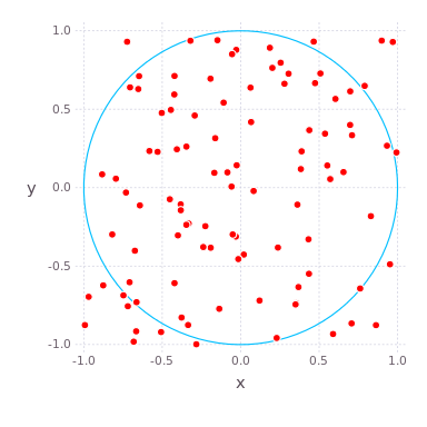
( , ) ( ) , , , . , , . compute_pi (N) , , .
function compute_pi(N::Int) # counts number of points that have radial coordinate < 1, ie in circle n_landed_in_circle = 0 for i = 1:N x = rand() * 2 - 1 # uniformly distributed number on x-axis y = rand() * 2 - 1 # uniformly distributed number on y-axis r2 = x*x + y*y # radius squared, in radial coordinates if r2 < 1.0 n_landed_in_circle += 1 end end return n_landed_in_circle / N * 4.0 end , , . : , , 25 .
Julia Pi.jl ( Sublime Text , ):
C:\Users\User\AppData\Local\Julia-1.1.0\bin\julia -p 4 julia> include("C:/Users/User/Desktop/Pi.jl") @everywhere function compute_pi(N::Int) n_landed_in_circle = 0 # counts number of points that have radial coordinate < 1, ie in circle for i = 1:N x = rand() * 2 - 1 # uniformly distributed number on x-axis y = rand() * 2 - 1 # uniformly distributed number on y-axis r2 = x*x + y*y # radius squared, in radial coordinates if r2 < 1.0 n_landed_in_circle += 1 end end return n_landed_in_circle / N * 4.0 end function parallel_pi_computation(N::Int; ncores::Int=4) # sum_of_pis = @distributed (+) for i=1:ncores compute_pi(ceil(Int, N / ncores)) end return sum_of_pis / ncores # average value end # ceil (T, x) # T, x. , :
julia> @time parallel_pi_computation(1000000000, ncores = 1) 6.818123 seconds (1.96 M allocations: 99.838 MiB, 0.42% gc time) 3.141562892 julia> @time parallel_pi_computation(1000000000, ncores = 1) 5.081638 seconds (1.12 k allocations: 62.953 KiB) 3.141657252 julia> @time parallel_pi_computation(1000000000, ncores = 2) 3.504871 seconds (1.84 k allocations: 109.382 KiB) 3.1415942599999997 julia> @time parallel_pi_computation(1000000000, ncores = 4) 3.093918 seconds (1.12 k allocations: 71.938 KiB) 3.1416889400000003 julia> pi ? = 3.1415926535897... JIT - — . , Julia . , ( Multi-Threading, Atomic Operations, Channels Coroutines).
useful links
, , . MPI.jl MPI ,
DistributedArrays.jl .
GPU, :
- ( C) OpenCL.jl CUDAdrv.jl OpenCL CUDA.
- ( Julia) CUDAnative.jl CUDA .
- , , CuArrays.jl CLArrays.jl
- , ArrayFire.jl GPUArrays.jl
- -
- Kynseed
, , . !

')
Source: https://habr.com/ru/post/455846/
All Articles