Brief Introduction to Markov Chains
In 1998, Lawrence Page, Sergey Brin, Rajiv Motvani and Terry Vinohrad published the article “The PageRank Citation Ranking: Bringing Order to the Web”, which now describes the famous PageRank algorithm, which became the foundation of Google. After a little less than two decades, Google has become a giant, and even though its algorithm has evolved greatly, PageRank is still a “symbol” of Google's ranking algorithms (although only a few people can really tell how much weight it takes today in an algorithm) .
From a theoretical point of view, it is interesting to note that one of the standard interpretations of the PageRank algorithm is based on a simple but fundamental concept of Markov chains. From the article we will see that Markov chains are powerful tools of stochastic modeling, which can be useful to any data analyst expert. In particular, we will answer such basic questions: what are Markov chains, what good properties do they have, and what can they do with their help?
Short review
In the first section, we give the basic definitions necessary to understand Markov chains. In the second section, we consider the special case of Markov chains in finite space of states. In the third section, we will look at some of the elementary properties of Markov chains and illustrate these properties in many small examples. Finally, in the fourth section, we will connect Markov chains with the PageRank algorithm and see in an artificial example how the Markov chains can be used to rank the nodes of a graph.
Note. To understand this post requires knowledge of the basics of probability and linear algebra. In particular, the following concepts will be used: conditional probability , eigenvector and formula of total probability .
What is a Markov chain?
Random variables and random processes
Before introducing the concept of Markov chains, let us briefly recall the basic, but important concepts of probability theory.
')
First, outside the language of mathematics, a random variable X is considered to be a quantity that is determined by the result of a random phenomenon. Its result can be a number (or “similarity of a number”, for example, vectors) or something else. For example, we can define a random variable as the result of a die roll (number) or as the result of a coin toss (not a number, unless we designate, for example, “eagle” as 0, and “tails” as 1). We also mention that the space of possible outcomes of a random variable can be discrete or continuous: for example, the normal random variable is continuous, and the Poisson random variable is discrete.
Next, we can define a random process (also called a stochastic process ) as a set of random variables indexed by the set T, which often denotes different points in time (in the future we will assume this way). The two most common cases: T can be either a set of natural numbers (a random process with discrete time) or a set of real numbers (a random process with continuous time). For example, if we throw a coin every day, we will define a random process with discrete time, and the ever-changing value of the option on the exchange will define a random process with continuous time. Random variables at different points in time can be independent of each other (an example with a coin toss), or have a certain dependence (an example with an option value); in addition, they can have a continuous or discrete space of states (the space of possible results at each moment of time).
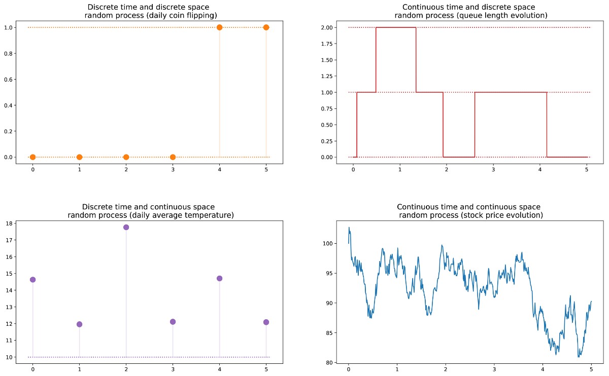
Different types of random processes (discrete / continuous in space / time).
Markov property and Markov chain
There are well-known families of random processes: Gaussian processes, Poisson processes, autoregressive models, moving average models, Markov chains, and others. Each of these individual cases has certain properties that allow us to better explore and understand them.
One of the properties that greatly simplifies the study of a random process is the “Markov property”. If we explain it in a very informal language, the Markov property tells us that if we know the value obtained by some random process at a given point in time, we will not get any additional information about the future behavior of the process, collecting other information about its past. More mathematical language: at any moment in time, the conditional distribution of future states of a process with given current and past states depends only on the current state, but not on past states (the absence of memory property ). A random process with a Markov property is called a Markov process .
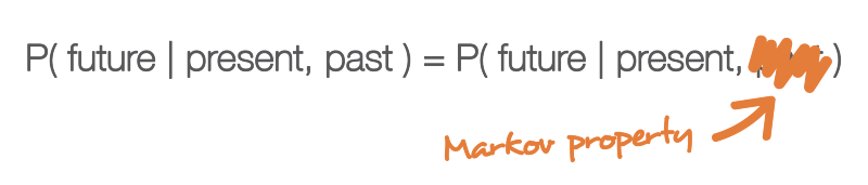
Markov property means that if we know the current state at a given point in time, then we do not need any additional information about the future, collected from the past.
Based on this definition, we can formulate the definition of “homogeneous Markov chains with discrete time” (hereinafter, for simplicity, we will call them “Markov chains”). A Markov chain is a Markov process with discrete time and a discrete state space. So, a Markov chain is a discrete sequence of states, each of which is taken from a discrete space of states (finite or infinite), satisfying the Markov property.
Mathematically, we can denote a Markov chain like this:

where at each moment of time the process takes its values from the discrete set E, such that

Then the Markov property implies that we have

Note again that this last formula reflects the fact that for chronology (where I am now and where I was before) the probability distribution of the next state (where I will be further) depends on the current state, but not on past states.
Note. In this introductory post, we decided to talk only about simple homogeneous Markov chains with discrete time. However, there are also non-uniform (time-dependent) Markov chains and / or chains with continuous time. In this article we will not consider such variations of the model. It is also worth noting that the definition of the Markov property given above is extremely simplified: the true mathematical definition uses the notion of filtering, which goes far beyond our introductory acquaintance with the model.
Characterize the dynamics of randomness of a Markov chain
In the previous section, we became acquainted with the general structure corresponding to any Markov chain. Let's see what we need to set a specific “instance” of such a random process.
First, we note that the complete determination of the characteristics of a random process with a discrete time that does not satisfy the Markov property can be a difficult task: the probability distribution at a given time can depend on one or several moments in the past and / or future. All of these possible temporal dependencies could potentially complicate the creation of a process definition.
However, due to the Markov property, the dynamics of a Markov chain are fairly easy to determine. And in fact. we only need to define two aspects: the initial probability distribution (that is, the probability distribution at time n = 0), denoted

and the transition probability matrix (which gives us the probability that the state at time n + 1 is the next for another state at time n for any pair of states), denoted

If these two aspects are known, then the full (probabilistic) dynamics of the process are clearly defined. Indeed, the probability of any outcome of the process can then be calculated cyclically.
Example: let's say we want to know the probability that the first 3 states of the process will have values (s0, s1, s2). So we want to calculate the probability

Here we apply the total probability formula, which states that the probability of obtaining (s0, s1, s2) is equal to the probability of obtaining the first s0 multiplied by the probability of obtaining s1, taking into account the fact that earlier we received s0 multiplied by the probability of obtaining s2 taking into account that we got earlier in order of s0 and s1. Mathematically, this can be written as

And then there is a simplification, determined by the Markov assumption. In fact, in the case of long chains, we obtain strongly conditional probabilities for the last states. However, in the case of Markov chains, we can simplify this expression by using the fact that

getting this way

Since they fully characterize the probabilistic dynamics of the process, many complex events can be calculated only on the basis of the initial probability distribution q0 and the transition probability matrix p. It is also worth giving one more basic connection: the expression of the probability distribution at time n + 1, expressed relative to the probability distribution at time n

Markov chains in finite state spaces
Representation in the form of matrices and graphs
Here we assume that in the set E there is a finite number of possible states N:

Then the initial probability distribution can be described as a vector-string q0 of size N, and the transition probabilities can be described as a matrix p of size N by N, such that

The advantage of such a record is that if we denote the distribution of probabilities at step n by the row vector qn, such that its components are specified

then simple matrix links are saved.

(here we will not consider the evidence, but it is very simple to reproduce it).
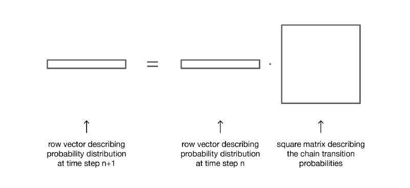
If we multiply to the right a row vector describing the distribution of probabilities at a given time, by a matrix of transition probabilities, we get the probability distribution at the next time.
So, as we see, the transition of the probability distribution from a given stage to the next is simply defined as the right multiplication of the probability vector row of the original step by the matrix p. In addition, this implies that we have

The dynamics of randomness of a Markov chain in finite state space can be easily represented as a normalized oriented graph, such that each node of the graph is a state, and for each pair of states (ei, ej) there is an edge going from ei to ej, if p (ei, ej )> 0. Then the value of the edge is the same probability p (ei, ej).
Example: reader of our site
Let's illustrate it all with a simple example. Consider the daily behavior of a fictional site visitor. Every day he has 3 possible states: the reader does not visit the site that day (N), the reader visits the site but does not read the entire post (V) and the reader visits the site and reads the whole post (R). So, we have the following state space:

Suppose, on the first day, this reader has a 50% chance only to enter the site and a 50% chance to visit the site and read at least one article. The vector describing the initial probability distribution (n = 0) then looks like this:

Also imagine that the following probabilities are observed:
- when the reader does not visit one day, he has a 25% chance of not visiting him and the next day, the probability of 50% is only to visit him and 25% to visit and read the article
- when a reader visits the site one day, but does not read, it has a 50% chance to visit it again the next day and not read the article, and a 50% chance to visit and read
- when a reader visits and reads an article on one day, he has a 33% chance not to enter the next day (I hope this post will not give such an effect!) , a 33% chance only to visit the site and 34% to visit and read the article again
Then we have the following transition matrix:

From the previous section, we know how to calculate for this reader the probability of each state on the next day (n = 1)

The probabilistic dynamics of this Markov chain can be represented graphically as:
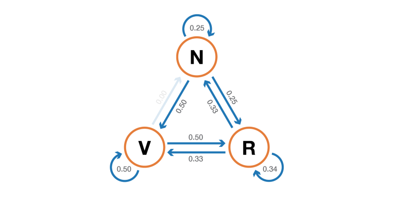
Representation in the form of a graph of a Markov chain, modeling the behavior of our invented site visitor.
Markov Chain Properties
In this section, we will discuss only some of the most basic properties or characteristics of Markov chains. We will not go into mathematical details, but present a brief overview of interesting points that need to be explored in order to use Markov chains. As we have seen, in the case of a finite space of states, the Markov chain can be represented as a graph. In the following, we will use a graphical representation to explain some properties. However, one should not forget that these properties are not necessarily limited to the case of a finite state space.
Degradability, periodicity, irrevocability and recoverability
In this subsection, let's start with a few classic ways of characterizing a state or a whole Markov chain.
First, we mention that the Markov chain is indecomposable if it is possible to reach any state from any other state (it is not necessary that in one time step). If the state space is finite and the chain can be represented as a graph, then we can say that the graph of an indecomposable Markov chain is strongly connected (graph theory).
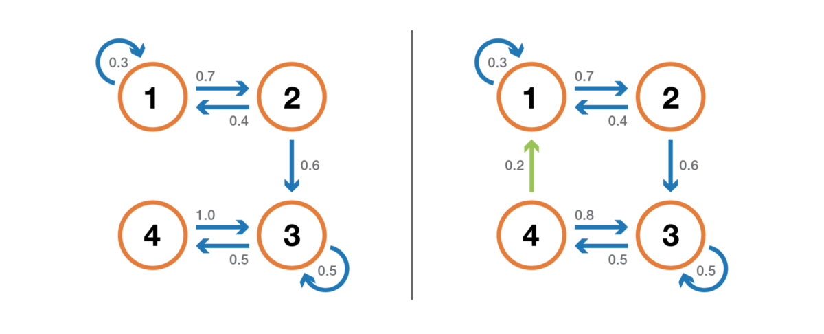
Illustration of the property of indecomposability (incompatibility). The chain on the left cannot be cut: from 3 or 4 we cannot get into 1 or 2. The chain on the right (one edge added) can be cut: each state can be reached from any other.
A state has a period k, if, when leaving it, any return to this state requires a number of stages of time, a multiple of k (k is the greatest common divisor of all possible lengths of return paths). If k = 1, then they say that the state is aperiodic, and the whole Markov chain is aperiodic if all its states are aperiodic. In the case of an irreducible Markov chain, it can also be mentioned that if one state is aperiodic, then all the others are also aperiodic.
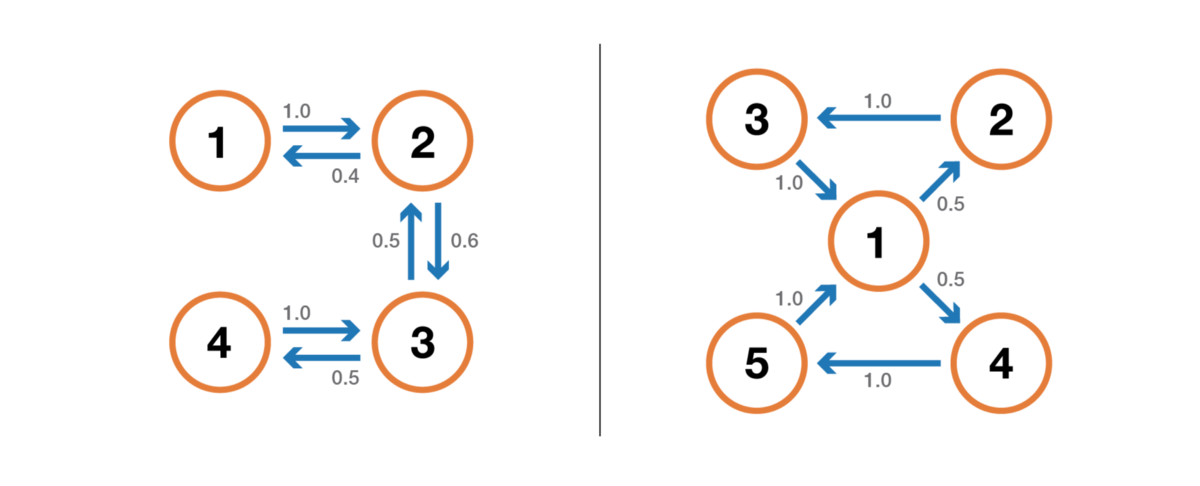
Illustration of the periodicity property. The chain on the left is periodic with k = 2: when leaving any state, the number of steps in a multiple of 2 is always required to return to it. The chain on the right has a period of 3.
A state is irrevocable if, upon leaving the state, there is a nonzero probability that we will never return to it. Conversely, a state is considered recurring if we know that after leaving the state we can return to it in the future with a probability of 1 (if it is not irretrievable).
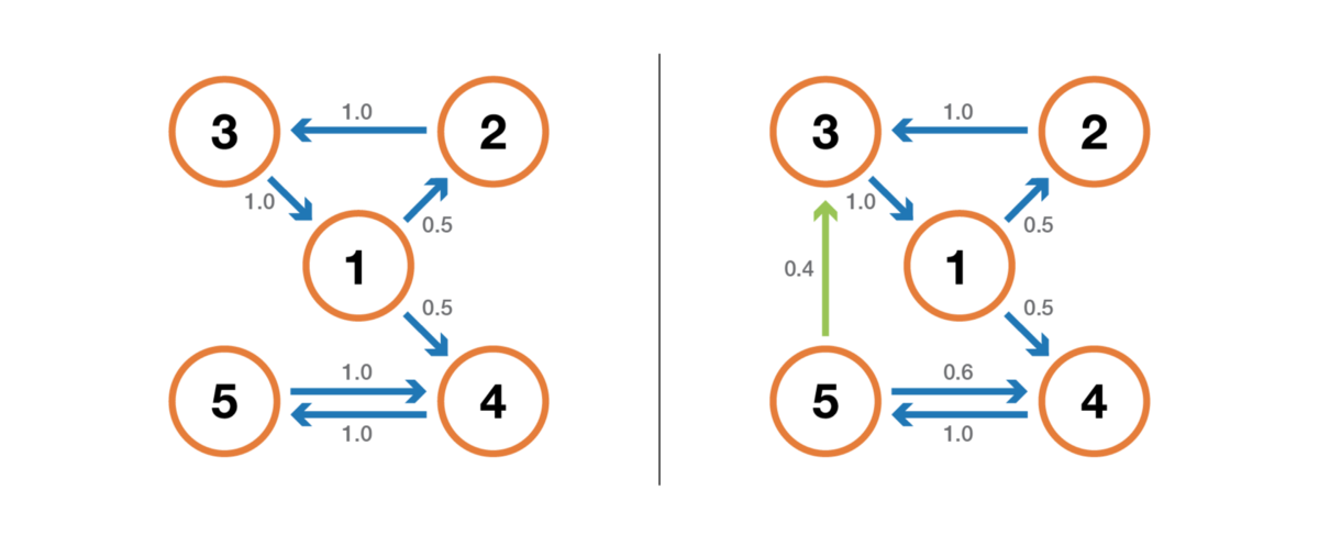
Illustration of the property of return / irrevocability. The chain on the left has the following properties: 1, 2 and 3 are non-returnable (when leaving these points we cannot be absolutely sure that we will return to them) and have period 3, and 4 and 5 are returnable (when leaving these points we are absolutely sure that one day we shall return to them) and have period 2. The chain on the right has one more edge, making the whole chain recurrent and aperiodic.
For the return state, we can calculate the average return time, which is the expected return time when leaving the state. Note that even the probability of return is 1, this does not mean that the expected return time is of course. Therefore, among all return states, we can distinguish between positive return states (with a finite expected return time) and zero return states (with an infinite expected return time).
Stationary distribution, limiting behavior and ergodicity
In this subsection, we consider the properties that characterize some aspects of the (random) dynamics described by the Markov chain.
The probability distribution π over the state space E is called a stationary distribution if it satisfies the expression

Since we have

Then the stationary distribution satisfies the expression

By definition, the stationary probability distribution does not change with time. That is, if the initial distribution q is stationary, then it will be the same at all subsequent stages of time. If the state space is finite, then p can be represented as a matrix, and π - as a row vector, and then we get

This again expresses the fact that the stationary probability distribution does not change with time (as we can see, multiplying the probability distribution by p on the right allows us to calculate the probability distribution at the next time step). Note that an indecomposable Markov chain has a stationary probability distribution if and only if one of its states is positive recurrent.
Another interesting property related to the stationary probability distribution is as follows. If the chain is positive returnable (that is, there is a stationary distribution in it) and aperiodic, then whatever the initial probabilities are, the probability distribution of the chain converges as the time intervals tend to infinity: they say that the chain has a limit distribution , which is nothing else as a stationary distribution. In general, it can be written as:

Once again, we emphasize the fact that we make no assumptions about the initial probability distribution: the probability distribution of a chain is reduced to a stationary distribution (an equilibrium distribution of a chain), regardless of the initial parameters.
Finally, ergodicity is another interesting property related to the behavior of the Markov chain. If a Markov chain is indecomposable, then it is also said that it is “ergodic” because it satisfies the following ergodic theorem. Suppose we have a function f (.), Going from the state space E to the axis (this can be, for example, the price of being in each state). We can determine the average value that moves this function along a given trajectory (temporary average). For nth first terms, this is denoted as

We can also calculate the average value of the function f on the set E, weighted by the stationary distribution (spatial average), which is denoted

Then the ergodic theorem tells us that when the trajectory becomes infinitely long, the temporal average is equal to the spatial average (weighted by the stationary distribution). The ergodicity property can be written as:

In other words, it means that in the previous limit, the behavior of the trajectory becomes insignificant and only the long-term stationary behavior is important in the calculation of the time average.
Let's return to the example with the reader of the site.
Consider again an example with a site reader. In this simple example, it is obvious that a chain is indecomposable, aperiodic, and all its states are positively reflexive.
To show what interesting results can be calculated using Markov chains, we consider the average return time to the state R (the state “visits the site and reads the article”). In other words, we want to answer the following question: if our reader comes to the site one day and reads an article, how many days will we have to wait on average for what he will come back and read the article? Let's try to get an intuitive understanding of how this value is calculated.
First we denote

So we want to calculate m (R, R). Arguing about the first interval reached after exiting from R, we get

However, this expression requires that we know m (N, R) and m (V, R) to calculate m (R, R). These two values can be expressed in a similar way:

So, we got 3 equations with 3 unknowns and after solving them we get m (N, R) = 2.67, m (V, R) = 2.00 and m (R, R) = 2.54. The value of the average return time to the state R is then 2.54. That is, using linear algebra, we were able to calculate the average return time to the state R (as well as the average transition time from N to R and the average transition time from V to R).
To finish with this example, let's see what the stationary distribution of the Markov chain will be. To determine the stationary distribution, we need to solve the following equation of linear algebra:

That is, we need to find the left eigenvector p associated with the eigenvector 1. Solving this problem, we obtain the following stationary distribution:
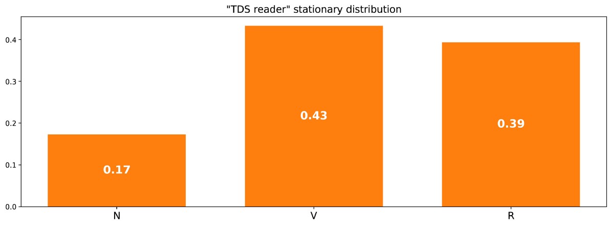
Stationary distribution in the example of the reader site.
It can also be noted that π (R) = 1 / m (R, R), and if we reflect a bit, then this identity is quite logical (but we will not discuss this in detail).
Since the chain is indecomposable and aperiodic, this means that in the long run the probability distribution will converge to a stationary distribution (for any initial parameters). In other words, whatever the initial state of the site reader, if we wait a long time and randomly choose a day, we get the probability π (N) that the reader will not enter the site that day, the probability π (V) that the reader will enter, but will not read the article, and the probability π® that the reader will enter and read the article. To better understand the convergence property, let's take a look at the following graph showing the evolution of probability distributions starting from different starting points and (rapidly) converging to a stationary distribution:
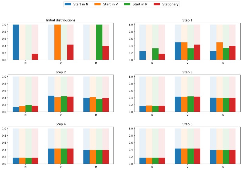
Visualization of the convergence of 3 probability distributions with different initial parameters (blue, orange and green) to the stationary distribution (red).
Classic example: PageRank algorithm
It's time to go back to PageRank! But before proceeding further, it is worth mentioning that the interpretation of PageRank given in this article is not the only possible one, and the authors of the original article did not necessarily count on the use of Markov chains when developing the methodology. However, our interpretation is good because it is very understandable.
Arbitrary web user
PageRank tries to solve the following problem: how do we rank the existing set (we can assume that this set has already been filtered, for example, by some query) with the help of the links that already exist between the pages?
To solve this problem and be able to rank the pages, PageRank roughly performs the following process. We believe that an arbitrary Internet user is located on one of the pages at the initial moment of time. Then this user starts randomly moving by clicking on each page one of the links that lead to another page of the set in question (it is assumed that all links leading outside of these pages are prohibited). On any page, all valid links have the same probability of being clicked.
So we set the Markov chain: pages are possible states, transition probabilities are set by links from page to page (weighted in such a way that on each page all related pages have the same probability of choice), and the lack of memory properties are clearly defined by the user's behavior. If we also assume that the given chain is positively recurrent and aperiodic (small tricks are applied to meet these requirements), then in the long run the probability distribution of the “current page” converges to a stationary distribution. That is, whatever the initial page, after a long time each page has a probability (almost fixed) to become current if we choose a random moment of time.
PageRank is based on the following hypothesis: the most likely pages in the stationary distribution should also be the most important (we visit these pages often because they receive links from pages that are also frequently visited during the transition). Then the stationary probability distribution determines the PageRank value for each state.
Artificial example
To make this much clearer, let's consider an artificial example. Suppose we have a tiny website with 7 pages, labeled from 1 to 7, and the links between these pages correspond to the next column.
For the sake of clarity, the probabilities of each transition are not shown in the animation shown above. However, since it is understood that “navigation” should be exclusively random (this is called “random walk”), the values can be easily reproduced from the following simple rule: for a node with K outgoing links (a page with K links to other pages), the probability of each outgoing link equals 1 / k. That is, the transition probability matrix has the form:

where 0.0 values are replaced by “.” for convenience. Before performing further calculations, we can notice that this Markov chain is indecomposable and aperiodic, that is, in the long run the system converges to a stationary distribution. As we saw, we can calculate this stationary distribution by solving the following left eigenvector problem

By doing this, we get the following PageRank values (stationary distribution values) for each page.
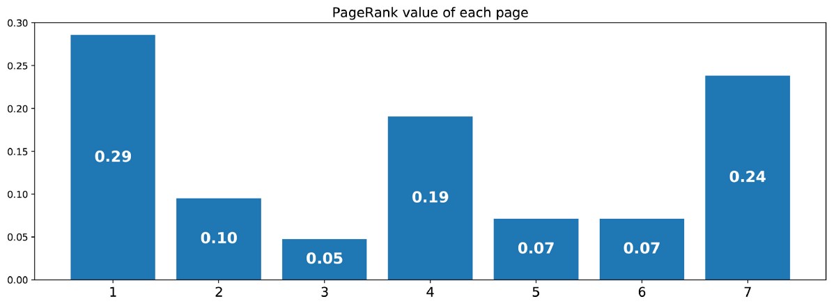
The PageRank values calculated for our artificial example of 7 pages.
Then the PageRank ranking of this tiny website looks like 1> 7> 4> 2> 5 = 6> 3.
findings
The main conclusions of this article are:
- random processes are sets of random variables, often indexed by time (indices often denote discrete or continuous time)
- for a random process, a Markov property means that for a given current, the probability of the future does not depend on the past (this property is also called “no memory”)
- discrete-time Markov chain are random processes with discrete-time indices that satisfy the Markov property
- ( , …)
- PageRank ( ) -, ; ( , , , )
In conclusion, we emphasize once again how powerful the Markov chains are in modeling problems associated with random dynamics. Due to their good properties, they are used in various fields, for example, in queuing theory (optimization of the performance of telecommunication networks, in which messages often have to compete for limited resources and are queued when all resources are already occupied), in statistics (well-known Monte Carlo methods). Carlo is based on the Markov chain for generating random variables based on Markov chains), in biology (modeling the evolution of biological populations), in computer science (hidden Markov models are important tools umentami in information theory, and speech recognition), as well as in other areas.
Of course, the enormous possibilities offered by Markov chains from the point of view of modeling and computation are much wider than those considered in this modest review. Therefore, we hope that we have been able to arouse the reader’s interest in the further study of these tools, which occupy an important place in the arsenal of the scientist and data expert.
Source: https://habr.com/ru/post/455762/
All Articles