On the application of parametric spectral estimation methods in radar - the method MUSIC. Addition to the article
I got a good article about the spectral estimation method, which is great for a short signal from the sum of low noise harmonics. (-copy) Perhaps my comments will help the reader understand the essence of the method. What is a little upsetting, it is not fully implemented features of the method. The method is applied to radar - to quickly determine the direction to incoming signals (angle θ) with the subsequent goal of an automatic, it should be understood, adaptation of the system. But - the author does not make a numerical definition of this angle (and this is strange in the context), although this definition is quite possible. We have only beautiful graphics, according to which, it turns out, the system must also be “crawled” and “crawled”, determining the number and location of the maxima, which is not entirely good.
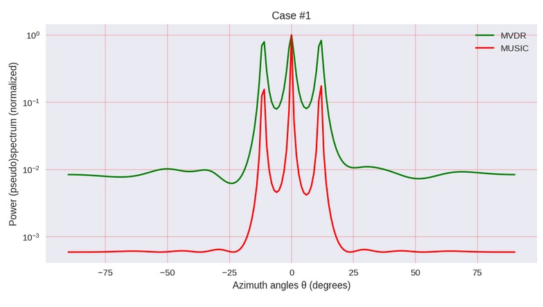
Illustration of the author of the mentioned article
"Formulation of the problem"
In short: we need to somehow determine from where (at what angle) the signal comes to the trellis antenna. Then to adjust it in the direction - but this is no longer in this “song”.
')
"Modeling of the received signal"
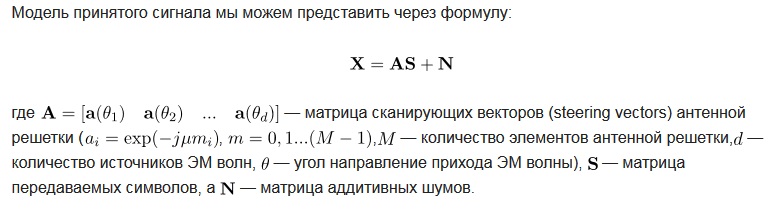
(it doesn't matter - apparently, the “symbol” should be read everywhere as a “signal”)
Here - be careful. The author seems to work with some kind of complex signal (spatial). Although X , yes, could be, as it is written, a matrix of “complex amplitudes” (depend not on the coordinate, but on the spatial frequency), but, for example, XX H is “covariances”, and not “spectral densities”.
The complex amplitude matrix is more like S , with which harmonic components (useful signal) are modeled. Neither additive noise, nor, it seems, even harmonic components are an analytical signal here. Although harmonics, with reservations, are very close to this.
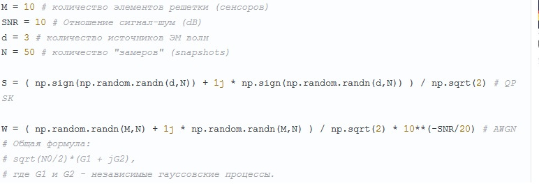
“# General formula:
# sqrt (N0 / 2) * (G1 + jG2),
# where G1 and G2 are independent Gaussian processes. ”
The main thing is where the imaginary component will appear from the real measurements, is somehow incomprehensible. Calculate the analytical signal at least in principle possible.
It is possible that there is a “primary source”, where they worked with valid X (received signal). For example, the author seems to be very eager to “make” the obtained spectra symmetric (even) - in all the considered cases, the test signals are given by the incoming signals symmetrically on the left and right.
"Conditions"
We determined the range of angles θ of the arrival of the signal, in which it makes sense to look. True, then the graphics are still building for some reason from +90 to -90 degrees.
"A bit of theory about the method itself"
Addition. MUSIC is obtained from the autoregressive estimation (from the Yule-Walker equations) practically by itself, in case the dispersion of the conditional white noise is negligible. The results are almost the same. The SLAE solution is even more economical than the search for eigenvectors, but, by the way, for several reasons spectral decomposition of a covariance matrix with its poor conditionality would be very desirable to produce anyway.
EVD, in general, is simply = “finding eigenvalues and vectors,” and nothing more. Not an algorithm.
Why do we write “pseudospectrum” - because we can only determine the spectrum from the eigenvectors of the covariance (correlation) matrix only up to a scale factor, i.e. the absolute values obtained do not make sense. But we need precisely and only the position of the maxima.
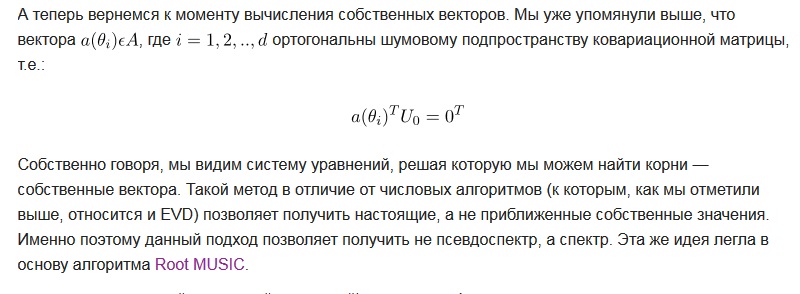
- This is the most interesting. Well, firstly, U 0 is already an eigenvector, only for the covariance matrix - and “saving” on their search will not work. Further. The search for solutions will lead to the necessity of determining the roots of a power equation, which is absolutely equivalent to another spectral decomposition. The author, apparently, confuses the eigenvalues of completely different matrices.
But ... the main thing ... now (!), Finally (!), We could logarithm the roots, numerically determine the complex "impedances" (model poles) (in the equation this is again θ, which is not very good) that we its imaginary part will show this very angle at which the signal came. Here it is a pity that the author did not.
"Modeling"
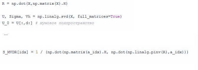
This is a little alarming - at first, the covariance matrix R = XX H was calculated, for which, for some reason, they immediately forgot for some time and started everything again - we decompose into singular numbers and vectors X. They promised something by text — look for the eigenvalues and the vectors of R, which, of course, is the same, but it would seem more logical when R has already been found. It is not clear what problem the author faced.
We remember about R when we estimate the spectrum using the MVDR dispersion minimum method. And here it is also interesting - R , judging by the script, seems to have been converted, in full accordance with this method, in a classical way, without any SVD (pseudo-inverse), although it seems to be low-ranking (strongly degenerate). In a sense, the noise is not that small? Well, maybe.
Actually, that's what confuses me. The size of the “noise subspace” in the script seems to be determined by a volitional order (equal to d). And we in the real case do not know how many harmonics are in the signal, and how much noise. It was necessary to analyze these eigenvalues - which of them are negligible, which of them are not.
In general, the work is very interesting, and not only for radar. The method, I believe, has great potential, precisely for such types of signal. The author worked very well, and some annoying inconsistencies are not so difficult to fix. And the main thing is to add an article using the RootMUSIC method.
Illustration of the author of the mentioned article
"Formulation of the problem"
In short: we need to somehow determine from where (at what angle) the signal comes to the trellis antenna. Then to adjust it in the direction - but this is no longer in this “song”.
')
"Modeling of the received signal"
(it doesn't matter - apparently, the “symbol” should be read everywhere as a “signal”)
Here - be careful. The author seems to work with some kind of complex signal (spatial). Although X , yes, could be, as it is written, a matrix of “complex amplitudes” (depend not on the coordinate, but on the spatial frequency), but, for example, XX H is “covariances”, and not “spectral densities”.
The complex amplitude matrix is more like S , with which harmonic components (useful signal) are modeled. Neither additive noise, nor, it seems, even harmonic components are an analytical signal here. Although harmonics, with reservations, are very close to this.
“# General formula:
# sqrt (N0 / 2) * (G1 + jG2),
# where G1 and G2 are independent Gaussian processes. ”
The main thing is where the imaginary component will appear from the real measurements, is somehow incomprehensible. Calculate the analytical signal at least in principle possible.
It is possible that there is a “primary source”, where they worked with valid X (received signal). For example, the author seems to be very eager to “make” the obtained spectra symmetric (even) - in all the considered cases, the test signals are given by the incoming signals symmetrically on the left and right.
"Conditions"
We determined the range of angles θ of the arrival of the signal, in which it makes sense to look. True, then the graphics are still building for some reason from +90 to -90 degrees.
"A bit of theory about the method itself"
Addition. MUSIC is obtained from the autoregressive estimation (from the Yule-Walker equations) practically by itself, in case the dispersion of the conditional white noise is negligible. The results are almost the same. The SLAE solution is even more economical than the search for eigenvectors, but, by the way, for several reasons spectral decomposition of a covariance matrix with its poor conditionality would be very desirable to produce anyway.
EVD, in general, is simply = “finding eigenvalues and vectors,” and nothing more. Not an algorithm.
Why do we write “pseudospectrum” - because we can only determine the spectrum from the eigenvectors of the covariance (correlation) matrix only up to a scale factor, i.e. the absolute values obtained do not make sense. But we need precisely and only the position of the maxima.
- This is the most interesting. Well, firstly, U 0 is already an eigenvector, only for the covariance matrix - and “saving” on their search will not work. Further. The search for solutions will lead to the necessity of determining the roots of a power equation, which is absolutely equivalent to another spectral decomposition. The author, apparently, confuses the eigenvalues of completely different matrices.
But ... the main thing ... now (!), Finally (!), We could logarithm the roots, numerically determine the complex "impedances" (model poles) (in the equation this is again θ, which is not very good) that we its imaginary part will show this very angle at which the signal came. Here it is a pity that the author did not.
"Modeling"
This is a little alarming - at first, the covariance matrix R = XX H was calculated, for which, for some reason, they immediately forgot for some time and started everything again - we decompose into singular numbers and vectors X. They promised something by text — look for the eigenvalues and the vectors of R, which, of course, is the same, but it would seem more logical when R has already been found. It is not clear what problem the author faced.
We remember about R when we estimate the spectrum using the MVDR dispersion minimum method. And here it is also interesting - R , judging by the script, seems to have been converted, in full accordance with this method, in a classical way, without any SVD (pseudo-inverse), although it seems to be low-ranking (strongly degenerate). In a sense, the noise is not that small? Well, maybe.
Actually, that's what confuses me. The size of the “noise subspace” in the script seems to be determined by a volitional order (equal to d). And we in the real case do not know how many harmonics are in the signal, and how much noise. It was necessary to analyze these eigenvalues - which of them are negligible, which of them are not.
In general, the work is very interesting, and not only for radar. The method, I believe, has great potential, precisely for such types of signal. The author worked very well, and some annoying inconsistencies are not so difficult to fix. And the main thing is to add an article using the RootMUSIC method.
Source: https://habr.com/ru/post/455393/
All Articles