How computers learned to recognize images incredibly well

A landmark scientific work from 2012 transformed the field of software image recognition

Today I can, for example, open Google Photos, write “the beach”, and see a bunch of my photos from various beaches that I have visited over the last decade. And I never signed my photos - Google recognizes beaches on them based on their content. This seemingly boring feature is based on the technology called “deep convolutional neural network”, which allows programs to understand images using a complex method that is inaccessible to technologies of previous generations.

In recent years, researchers have found that software accuracy becomes better as they create deeper neural networks (NNs) and train them on ever larger data sets. This created an insatiable need for computing power, and enriched GPU manufacturers such as Nvidia and AMD. A few years ago, Google developed its own special chips for the National Assembly, while other companies are trying to keep up with it.

In Tesla, for example, Andrei Karpati, an expert on deep learning, was appointed head of the Autopilot project. Now the automaker is developing its own chip to speed up the work of the National Assembly in future versions of the autopilot. Or take Apple: in the A11 and A12 chips, central to the latest iPhones, there is the Neural Engine “ neural processor ”, which accelerates the work of the National Assembly and allows the applications for image and voice recognition to work better.
')
The experts I interviewed for this article track the beginning of the depth learning boom to a specific work: AlexNet, named after its main author, Alex Krizhevsky. “I believe that 2012 was a landmark year when AlexNet’s work came out,” said Sean Gerrish, an MO expert and author of How Smart Machines Think .

Until 2012, deep neural networks (GNS) were something of a remote place in the world of MO. But then Krizhevsky and his colleagues from the University of Toronto filed an application for a prestigious competition in image recognition, and she radically surpassed in accuracy everything that was developed before her. Almost instantly, the HNS has become the leading technology in image recognition. Other researchers who used this technology soon demonstrated further improvements in recognition accuracy.

In this article, we delve into deep learning. I will explain what NS are, how they are taught, and why they require such computational resources. And then I will explain why a certain type of NA — deep convolutional networks — is so well understood by images. Do not worry, there will be a lot of pictures.

Simple example with one neuron

The concept of "neural network" may seem vague to you, so let's start with a simple example. Suppose you want the NA to decide whether the car should go, on the basis of green, yellow and red traffic lights. NA can solve this problem with a single neuron.



The neuron receives input data (1 is on, 0 is off), multiplies by the corresponding weight, and adds all the values ​​of the weights. Then the neuron adds an offset that defines the threshold value for the "activation" of the neuron. In this case, if the output is positive, we consider that the neuron is activated - and vice versa. The neuron is equivalent to the inequality "green - red - 0.5> 0". If it turns out to be true - that is, the green is on, and the red is off - then the car must go.

In a real NS, artificial neurons take another step. Summing the weighted input and adding the offset, the neuron applies a nonlinear activation function. Often used sigmoid, S-shaped function, always producing a value from 0 to 1.

Using the activation function will not change the result of our simple traffic light model (we just need to use a threshold value of 0.5, not 0). But the nonlinearity of the activation functions is necessary in order for the NNs to model more complex functions. Without the activation function, each arbitrarily complex NA is reduced to a linear combination of input data. A linear function can not simulate the complex phenomena of the real world. Nonlinear activation function allows the NA to approximate any mathematical function .

Network example

Of course, there are many ways to approximate a function. NNs are distinguished by the fact that we know how to “train” them using a little algebra, a bunch of data and a sea of ​​computing power. Instead of the programmer developing directly the NA for a specific task, we can create software that starts with a fairly common NA, examines a bunch of marked examples, and then modifies the NA so that it gives the correct label for as many examples as possible. The expectation is that the final NA will summarize the data and will issue the correct labels for examples that were not previously in the database.

The process leading to this goal began long before AlexNet. In 1986, a trio of researchers published a landmark work on backpropagation — a technology that helped make the mathematical teaching of complex NAs a reality.

To get an idea of ​​how backpropagation works, let's take a look at a simple NA described by Michael Nielsen in his excellent online GO tutorial . The purpose of the network is to process the image of a handwritten digit in the resolution of 28x28 pixels and correctly determine whether the digit is written 0, 1, 2, etc.

Each image is 28 * 28 = 784 input values, each of which is a real number from 0 to 1, indicating how bright or dark the pixel is. Nielsen created this type of NA:



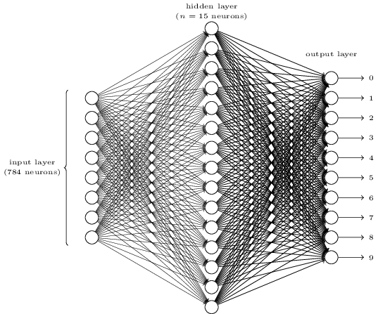
Each circle in the center and in the right column is a neuron, similar to the one we discussed in the previous section. Each neuron takes a weighted average of the input data, adds an offset, and applies an activation function. The circles on the left are not neurons, they denote network input data. And although the picture shows only 8 input circles, in fact there are 784 — one for each pixel.

Each of the 10 neurons on the right should “work” on its own number: the top one should turn on when handwritten 0 is input (and only in this case), the second one when the network sees handwritten 1 (and only her), and so on.

Each neuron perceives input from each neuron of the previous layer. So each of the 15 neurons in the middle receives 784 input values. Each of these 15 neurons has a weight parameter for each of the 784 input values. This means that only this layer has 15 * 784 = 11,760 weight parameters. Similarly, the output layer contains 10 neurons, each of which accepts input from all 15 neurons of the middle layer, which adds another 15 * 10 = 150 weight parameters. In addition, the network has 25 variable offsets - one for each of the 25 neurons.

Neural network training

The goal of the training is to adjust these 11 935 parameters to maximize the likelihood that the desired output neuron — and only he — is activated when the networks give an image of a handwritten digit. We can do this with the help of the famous MNIST image set, where there are 60,000 labeled images with a resolution of 28x28 pixels.


160 of 60,000 images from the MNIST set

Nielsen demonstrates how to train a network using 74 lines of regular python code - without any libraries for MO. Training begins with the selection of random values ​​for each of these 11 935 parameters, weights and offsets. The program then iterates over the sample images, going through two stages with each of them:

1. The forward propagation step calculates the network output based on the input image and current parameters.
2. The backward propagation step calculates the deviation of the result from the correct output data and modifies the network parameters so as to slightly improve its performance on the image.

Example. Suppose the network received the following image:



If it is well calibrated, then output “7” should tend to 1, and the other nine conclusions should tend to 0. But suppose that instead, the network at output “0” gives a value of 0.8. It's too much! The learning algorithm changes the input weights of the neuron responsible for "0", so that it gets closer to 0 the next time it processes this image.

For this, the backpropagation algorithm calculates the error gradient for each input weight. This is a measure of how the output error changes for a given change in input weight. Then the algorithm uses a gradient to decide how much to change each input weight - the larger the gradient, the stronger the change.

In other words, the learning process "teaches" the neurons of the output layer to pay less attention to those inputs (neurons in the middle layer) that push them to the wrong answer, and more to those inputs that push in the right direction.

The algorithm repeats this step for all other output neurons. It reduces the input weights for neurons "1", "2", "3", "4", "5", "6", "8" and "9" (but not "7") in order to lower the value of these output neurons. The higher the output value, the greater the gradient of the output error relative to the input weight - and the stronger its weight decreases.

Conversely, the algorithm increases the weight of the input data for output “7”, which causes the neuron to issue a higher value the next time it is given this image. Again, inputs with larger values ​​will increase the weight more, which will force the output neuron “7” to pay more attention to these inputs in the following times.

Then the algorithm must perform the same calculations for the middle layer: change each input weight in the direction that will reduce network errors - again, bringing the output “7” closer to 1, and the rest to 0. But each middle neuron has a connection with all 10 weekends, which complicates matters in two ways.

First, the error gradient for each average neuron depends not only on the input value, but also on the error gradients in the next layer. The algorithm is called backpropagation because the error gradients of the later layers of the network propagate in the opposite direction and are used to calculate gradients in the earlier layers.

Also, each middle neuron is an input for all ten weekends. Therefore, the learning algorithm has to calculate the error gradient, which reflects how a change in a certain input weight affects the average error across all outputs.

Back propagation is an algorithm for climbing a hill: each of its passes brings the output values ​​closer to the correct ones for a given image, but only a little. The more examples the algorithm scans, the higher it climbs up the hill, towards the optimal set of parameters that correctly classify the maximum number of training examples. Thousands of examples are required to achieve high accuracy, and the algorithm may need to cycle through each image in this set dozens of times before its efficiency stops growing.

Nielsen shows how to implement these 74 lines in python. Surprisingly, a network trained with such a simple program is able to recognize more than 95% of handwritten numbers from the MNIST database. With additional enhancements, a simple two-layer network is able to recognize more than 98% of the numbers.

AlexNet Breakthrough

You might think that the development of the theme of backward proliferation should have gone through in the 1980s, and to generate rapid progress in the Defense Ministry based on the National Assembly - but this did not happen. In the 1990s and the early 2000s, some people worked on this technology, but interest in the National Assembly did not gain momentum until the early 2010s.

This can be tracked by the results of the ImageNet competition - an annual competition in MO organized by a computer scientist from Stanford Fey-Fey Lee. Each year, opponents are given the same set of more than a million images for training, each of which is manually labeled in categories of more than 1000 - from the “fire engine” and “mushroom” to “cheetah”. Software participants are judged by the possibility of classifying other images that were not in the set. The program can give out several guesses, and its work is considered successful if at least one of the five first guesses coincides with the mark made by the person.

The competition began in 2010, and deep NAs did not play a big role in it in the first two years. The best teams used different MO techniques, and achieved rather average results. In 2010, the team won with an error rate of 28. In 2011, with an error of 25%.

And then came 2012. A team from the University of Toronto made a bid - which AlexNet was later christened in honor of the lead author of the work, Alex Krizhevsky - and left the rivals far behind. Using deep NA, the team achieved a 16% error rate. For the nearest competitor, this figure was 26.

The NS described in the article for handwriting recognition has two layers, 25 neurons and almost 12,000 parameters. AlexNet was much larger and more complex: eight trained layers, 650,000 neurons and 60 million parameters.

To train an NS of this size requires enormous computational power, and AlexNet has been designed to take advantage of the massive parallelization available on modern GPUs. The researchers thought of how to divide the network training work into two GPUs, which doubled the power. And still, despite the hard optimization, the network training took 5-6 days on the hardware that was available in 2012 (on a pair of Nvidia GTX 580 with 3 Gb of memory).

It is useful to study the examples of the results of AlexNet’s work in order to understand how serious this breakthrough was. Here is a picture from a scientific work, which shows examples of images and the first five network guesses according to their classification:



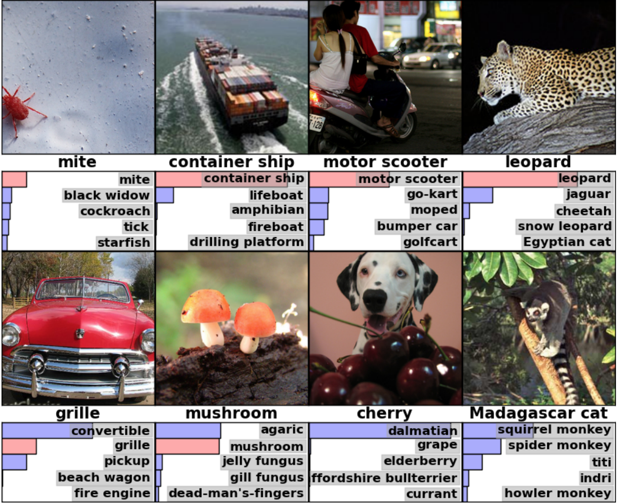
AlexNet was able to recognize on the first picture of the tick, although from it there is only a small form in the very corner. The software not only correctly identified the leopard, but also gave other close options - jaguar, cheetah, snow leopard, Egyptian mau. AlexNet tagged a photo of hornbeams as a “mushroom”. Just "mushroom" was the second version of the network.

AlexNet's “bugs” are also impressive. She noted a photo with a Dalmatian, standing behind a bunch of cherries, as "Dalmatian", although the official label was "cherry". AlexNet recognized that there was a berry in the photo - among the first five options were "grapes" and "elderberry" - she simply did not recognize the cherry. To a photo of a Madagascar lemur sitting in a tree, AlexNet has listed a list of small mammals living in trees. I think that many people (including me) would have put the wrong signature here.

The quality of work was impressive, and demonstrated that the software is able to recognize ordinary objects in a wide range of their orientations and environments. GNS quickly became the most popular technique for image recognition, and since then the world of MoD has not refused it.

“On the wave of success in 2012 of the method based on civil defense, most of the participants of the 2013 competition switched to deep convolutional neural networks,” wrote sponsors of ImageNet. In the following years, this trend continued, and subsequently the winners worked on the basis of basic technologies, first used by the AlexNet team. By 2017, rivals, using deeper NAs, seriously reduced the percentage of errors to less than three. Given the complexity of the problem, computers in some way have learned to solve it better than many people.


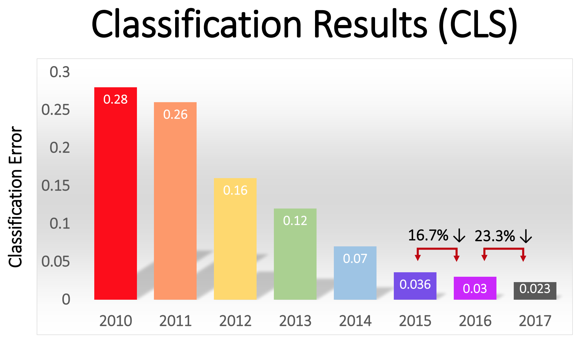
The percentage of errors in the classification of images in different years

Convolution networks: concept

Technically, AlexNet was a convolutional NA. In this section, I will explain what makes the convolutional neural network (SNS), and why this technology has become crucial for modern pattern recognition algorithms.

The previously considered simple handwriting recognition network was completely connected: each neuron of the first layer was an input for each neuron of the second layer. This structure works quite well on simple tasks with recognition of numbers on images of 28x28 pixels. But it doesn’t scale well.

In the MNIST handwritten digit database, all characters are centered. This seriously simplifies learning, since, let's say, the seven will always have several dark pixels at the top and right, and the bottom left corner is always white. Zero will almost always have a white spot in the middle and dark pixels along the edges. A simple and fully connected network can recognize such patterns fairly easily.

But, let's say, you wanted to create an NA capable of recognizing numbers that can be placed anywhere on a larger image. A fully connected network will not work just as well with such a task, since it does not have an effective way to recognize similar features of forms located in different parts of the image. If in your training dataset most of the sevens are located in the upper left corner, then your network will better recognize the sevens in the upper left corner than in any other part of the image.

Theoretically, this problem can be solved by ensuring that there are many examples of each digit in each of the possible positions in your set. But in practice it will be a huge waste of resources. With increasing image size and network depth, the number of links — and the number of weight parameters — will grow explosively. You will need much more training images (and computing power) to achieve adequate accuracy.

When a neural network learns to recognize a form located in one place of the image, it should be able to apply this knowledge to recognize the same form in other parts of the image. SNS provide an elegant solution to this problem.

“It’s like if you took a stencil and put it on all the places in the image,” said AI researcher Jai Ten. - You have a stencil with a dog image, and you first attach it to the upper right corner of the image to see if there is a dog there? If not, you move the stencil slightly. And so for the whole image. No matter where the picture of the dog is. Stencil will match with it. You do not need every part of the network to learn its own classification of dogs. ”

Imagine that we took a large image, and smashed into squares 28x28 pixels. Then we will be able to feed each small square of a fully connected web that recognizes handwriting, which we have studied before. If at least one of the squares will work output "7", it will be a sign that in general there is a seven in the image. This is what convolution networks do.

How convolution networks worked in AlexNet

In convolutional networks, such "stencils" are known as feature detectors, and the area they are studying is known by the receptive field. Real feature detectors work with much smaller margins than a square with a side of 28 pixels. In AlexNet, the feature detectors in the first convolutional layer worked with a receptive field of 11x11 pixels in size. In subsequent layers, receptive fields were 3-5 units wide.

In the process of traversing, the feature detector of the input image produces a feature map: a two-dimensional lattice on which it is noted how strongly the detector was activated in different parts of the image. Convolutional layers usually have more than one detector, and each of them scans an image in search of different patterns. AlexNet had 96 sign detectors on the first layer, which produced 96 sign cards.



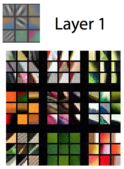
To better understand this, consider the visual representation of the patterns studied by each of the 96 detectors of the first AlexNet layer after network training. There are detectors looking for horizontal or vertical lines, transitions from light to dark, chess patterns and many other forms.

A color image is usually represented as a pixel map with three numbers for each pixel: the value of red, green, and blue. The first layer of AlexNet takes this representation and turns it into a representation using 96 numbers. Each “pixel” in this image has 96 values, one for each feature detector.

In this example, the first of 96 values ​​indicates whether some image point matches this pattern:



The second value indicates whether some image point coincides with this pattern:



The third value indicates whether some image point coincides with this pattern:



And so on for 93 more feature detectors in the first AlexNet layer. The first layer produces a new image representation, where each pixel is a vector in 96 dimensions (later I will explain that this representation is reduced 4 times).

Such is the first layer of AlexNet. Then there are four more convolutional layers, each of which accepts the output of the previous one as input.

As we have seen, the first layer detects basic patterns, such as horizontal and vertical lines, transitions from light to dark and curves. The second level uses them as a building block for recognizing slightly more complex forms. For example, the second layer could have a feature detector that finds circles using a combination of the outputs of the first layer feature detectors that find the curves. The third layer finds even more complex forms, combining features from the second layer. The fourth and fifth find even more complex patterns.

Researchers Matthew Seiler and Rob Fergus published an excellent work in 2014, which provides very useful ways to visualize patterns recognized by a five-layer neural network similar to ImageNet.

In the next slideshow, taken from their work, each image, except the first, has two halves. On the right, you will see examples of thumbnails that strongly activated a specific feature detector. They are collected by nine - and each group corresponds to its detector.On the left is a map showing which particular pixels in this miniature are most responsible for the coincidence. This is especially well seen on the fifth layer, because there are feature detectors that react strongly to dogs, logos, wheels, and so on.


First layer - simple patterns and forms


the second layer - begin to show fine structure


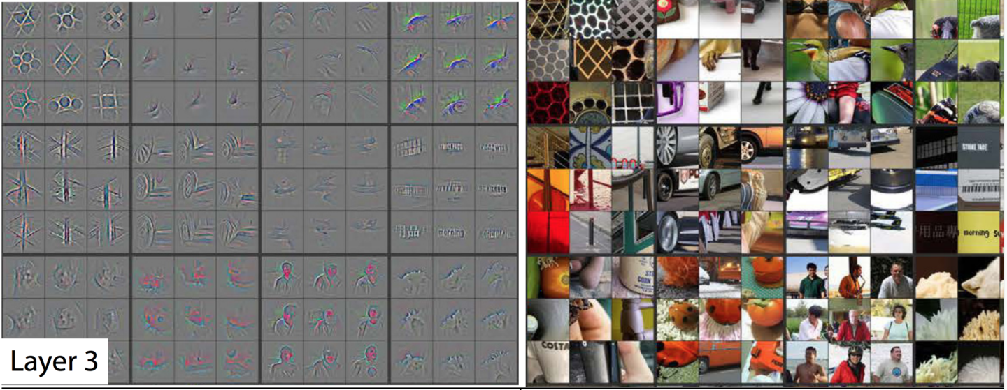
detectors signs on the third layer can recognize more complex shapes, such as the wheels of vehicles, cells and even people silhouettes


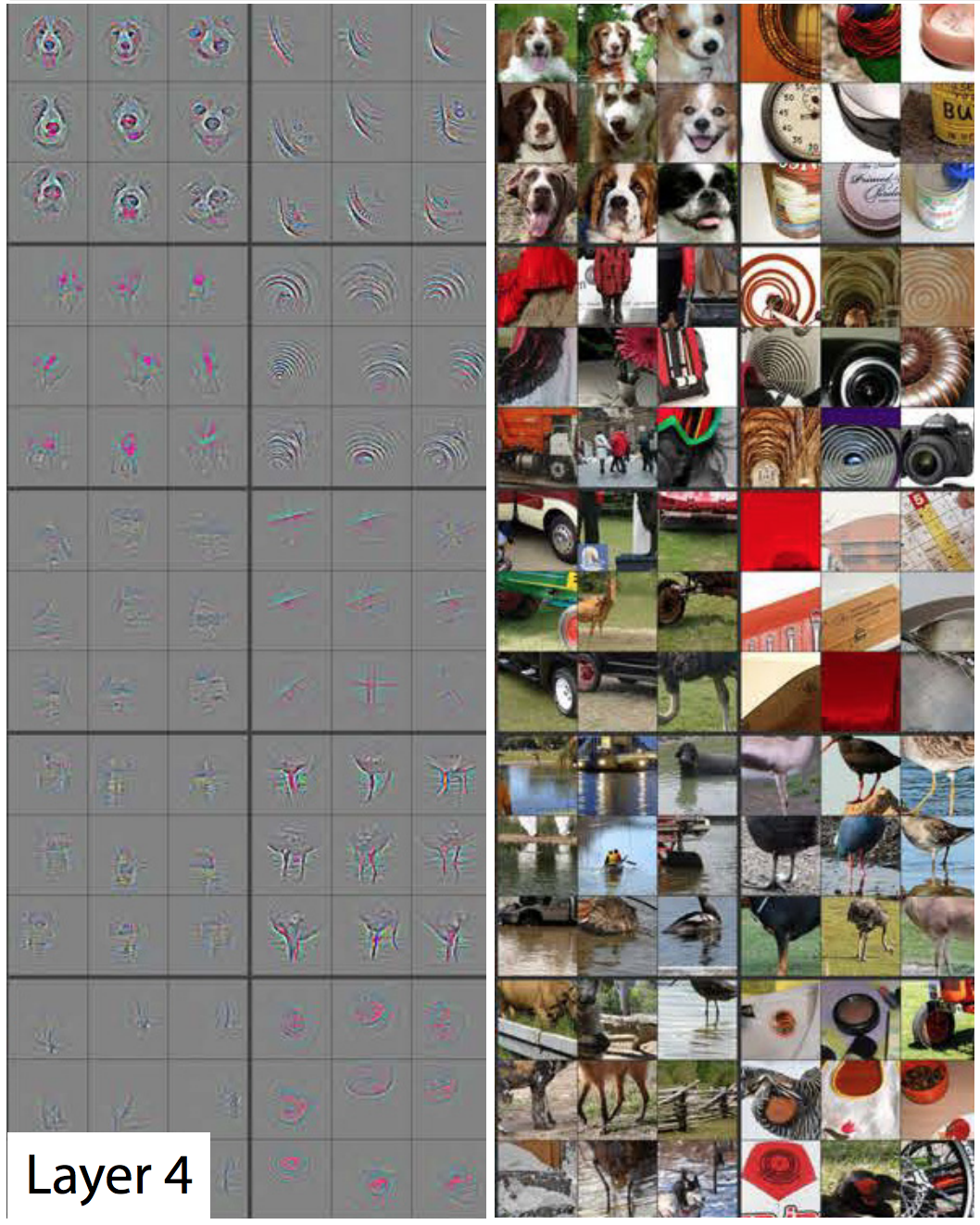
fourth layer is able to distinguish between complex shapes, such as mugs dogs or bird feet


fifth layer may recognize very complex shapes

Looking through the images, you can see how each subsequent layer is able to recognize more and more complex patterns. The first layer recognizes simple patterns that are not similar to anything. The second recognizes textures and simple shapes. By the third layer, recognizable shapes like wheels and red-orange spheres (tomatoes, ladybugs, something else) become visible.

In the first layer, the side of the receptive field is 11, and in the later, from three to five. But remember, later layers recognize feature maps generated by earlier layers, so each of their “pixels” means several pixels of the original image. Therefore, the receptive field of each layer includes a larger part of the first image than the previous layers. This is part of the reason that miniatures in later layers look more complicated than in earlier ones.

The fifth, last layer of the network is able to recognize an impressively large range of elements. For example, look at this image that I selected from the top right corner of the image corresponding to the fifth layer: The



nine pictures on the right may not look like each other. But if you look at the nine heat maps on the left, you will see that this feature detector does not concentrate on the objects in the foreground of the photos. Instead, it concentrates on the grass against the background of each!

Obviously, a grass detector is useful if one of the categories you are trying to determine is “grass”, but it can be useful for many other categories. After five convolutional layers, AlexNet has three layers that are fully connected, like our handwriting recognition network. These layers look at each of the feature maps produced by the five convolutional layers, trying to classify the image into one of 1000 possible categories.

So if there is grass in the background, then a wild animal will most likely appear on the image. On the other hand, if there is grass in the background, it is less likely to be the image of furniture in the house. These and other fifth layer feature detectors provide a lot of information about the likely photo content. The last layers of the network synthesize this information to produce a conjecture supported by the facts about what is generally shown in the picture.

What distinguishes convolutional layers: total input weights

We have seen that the feature detectors in convolutional layers exhibit impressive pattern recognition, but so far I have not explained how convolutional networks actually work.

The convolutional layer (SS) consists of neurons. They, like any neurons, take a weighted average per input and use the activation function. Parameters are trained using reverse propagation techniques.

But, unlike previous NA, the SS is not fully connected. Each neuron accepts input from a small fraction of the neurons from the previous layer. And, importantly, convolutional neurons have common input weights.

Let's consider the first neuron of the first SS AlexNet in more detail. The receptive field of this layer has a size of 11x11 pixels, so the first neuron examines the square of 11x11 pixels in one corner of the image. This neuron receives input data from this 121 pixels, and each pixel has three values ​​— red, green, and blue. Therefore, in general, the neuron has 363 input parameters. Like any neuron, this one takes a weighted average of 363 parameters, and applies an activation function to them. And, since the input parameters are 363, the weighting parameters also need 363.

The second neuron of the first layer is similar to the first. He also studies squares of 11x11 pixels, but his receptive field is shifted four pixels from the first. Two fields have an overlap of 7 pixels, so the network does not lose sight of interesting patterns that fall at the junction of two squares. The second neuron also takes 363 parameters describing a 11x11 square, multiplies each of them by weight, adds and applies an activation function.

But instead of using a separate set of 363 weights, the second neuron uses the same weights as the first. The top left pixel of the first neuron uses the same weights as the top left pixel of the second. Therefore, both neurons are looking for the same pattern; just their receptive fields are shifted 4 pixels relative to each other.

Naturally, there are more than two neurons there: 3025 neurons are in the 55x55 grid. Each of them uses the same set of 363 weights as the first two. Together, all neurons form a feature detector, a “scanning” image for the desired pattern, which can be located anywhere.

Remember that the first AlexNet layer has 96 feature detectors. The 3025 neurons I just mentioned constitute one of these 96 detectors. Each of the other 95s is a separate group of 3025 neurons. Each group of 3025 neurons uses a common set of 363 scales - however, for each of the 95 groups it has its own.

SNs are trained using the same backward propagation that is used for fully connected networks, but the convolutional structure makes the learning process more efficient and effective.

“The use of bundles really helps - the parameters can be reused,” the MO expert and author Sean Gerrish told us. This drastically reduces the number of input weights that a network has to learn, which allows it to produce better results with fewer teaching examples.

Training on one part of the image translates into improved recognition of the same pattern in other parts of the image. This allows the network to achieve high performance on a much smaller number of training examples.

People quickly realized the power of deep convolutional networks

AlexNet's work became a sensation in the academic community of the MoD, but its importance was quickly understood in the IT industry. She became particularly interested in Google.

In 2013, Google acquired a startup founded by the authors of AlexNet. The company used this technology to add new photo search feature in Google Photos. “We took an advanced study and launched it in a little more than six months,” wrote Chuck Rosenberg of Google.

Meanwhile, in the work of 2013, it was described how Google uses the GSS for recognizing addresses from Google Street View photos. “Our system helped us extract nearly 100 million physical addresses from these images,” the authors wrote.

The researchers found that the effectiveness of the NA increases with increasing depth. “We found that the effectiveness of this approach grows with increasing depth of the SNS, and the best results show the deepest of all the architectures we have trained,” wrote the Google Street View team. “Our experiments suggest that deeper architectures can produce greater accuracy, but with a slower increase in efficiency.”

So after AlexNet, the networks started to get deeper. The Google team came up with a winning bid in 2014 — just two years after AlexNet won in 2012. It was also based on deep SNS, but Goolge used a much deeper network of 22 layers to achieve an error rate in 6.7% - this was a significant improvement compared with 16% for AlexNet.

But at the same time, deeper networks worked better only with larger sets of training data. Therefore, Gerrish said that the ImageNet data set and the competition played a major role in the success of the SNA. Recall that in an ImageNet competition, participants are given a million images each and asked to sort them into 1000 categories.

“If you have a million images to learn, then each class includes 1000 images,” said Gerrish. Without such a large data set, he said, “you would have too many parameters for network training.”

In recent years, experts have increasingly focused on collecting a huge amount of data for learning deeper and more accurate networks. That is why companies developing robomobils concentrate on running along public roads — images and videos of these trips are sent to headquarters and used to train corporate NAs.

Computational deep learning boom

The discovery of the fact that deeper networks and more voluminous data sets can improve the performance of the NA has created an insatiable thirst for ever-increasing computing power. One of the main components of AlexNet’s success was the idea that matrix operations are used in NA training, which can be effectively performed on well-parallelized graphics processors.

“The National Assembly is well parallelized,” said a researcher in the field of Defense Jai Ten. Graphic cards - providing enormous parallel computing power for video games - have proven to be useful for NN as well.

"The central part of the work of the GPU, the very fast matrix multiplication, turned out to be the central part for the work of the National Assembly," said Ten.

All this was successful for the leading manufacturers of GPU, Nvidia and AMD. Both companies have developed new chips specifically tailored to the needs of MO applications, and now AI applications are responsible for a significant portion of the GPU sales of these companies.

In 2016, Google announced the creation of a special chip, the Tensor Processing Unit (TPU), designed to operate the National Assembly. “Although Google considered the possibility of creating special-purpose integrated circuits (ASIC) back in 2006, this situation became urgent in 2013,” a company spokesman wrote last year. “It was then that we realized that the rapidly growing NS requirements for computing power may require us to double the number of data centers we have.”

At first, only Google’s own services had access to TPU, but later the company allowed everyone to use this technology through a cloud computing platform.

Of course, Google is not the only company working on AI chips. Just a few examples: in the latest versions of chips for the iPhone there is a “neural core” optimized for operations with NA. Intel is developing its own line of chips optimized for GO. Tesla recently announced the failure of Nvidia's chips in favor of its own NS chips. Amazon is also rumored to be working on its own AI chips.

Why deep neural networks are hard to understand

I explained how neural networks work, but did not explain why they work so well. It is rather incomprehensible how exactly an immense amount of matrix calculations allows a computer system to distinguish a jaguar from a cheetah, and an elderberry from a currant.

Perhaps the most remarkable quality of the NA is that they do not. Convolutions allow the NA to understand hyphenation - they can tell whether the picture from the upper right corner of the image is similar to the image in the upper left corner of another image.

But at the same time, the SNA has no idea about geometry. They cannot recognize the similarity of two pictures if they are rotated 45 degrees or doubled. SNA does not try to understand the three-dimensional structure of objects, and can not take into account different lighting conditions.

But at the same time, NSs can recognize photos of dogs taken both from the front and from the side, and it does not matter whether the dog occupies a small part of the image, or a large one. How do they do it?It turns out that with enough data available, the statistical brute force approach can do the job. SNA is not designed so that it can “present” how a certain image would look from another angle or in other conditions, but with a sufficient number of marked examples, it can learn all possible variants of the image by simple repetition.

There is evidence that the visual system of people works in a similar way. Look at a couple of pictures - first carefully examine the first one, and then open the second one.


First photo



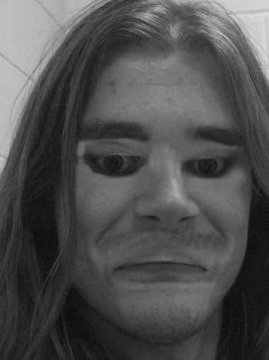
The creator of the image took someone's photo and turned his eyes and mouth upside down. The picture seems relatively normal when you look at it upside down, because the human visual system is used to seeing the eyes and mouths in this position. But if you look at the picture in the correct orientation, it is immediately clear that the face is strangely distorted.

This suggests that the human visual system is based on the same coarse techniques for recognizing patterns as NA. If we look at something that is almost always seen in one orientation - the human eye - we can recognize it much better in its normal orientation.

NAs recognize images well, using all the context available to them. For example, cars usually drive on roads. Dresses are usually put on the body of a woman or hang in the closet. Planes are usually shot against the sky or they are driving along the runway. Nobody specifically teaches the National Assembly with these correlations, but with a sufficient number of marked examples, the network itself can learn them.

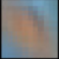
In 2015, researchers from Google tried to better understand the NA, “launching them backwards”. Instead of using pictures to teach the NA, they used trained NAs to change the pictures. For example, they started with an image containing random noise, and then gradually changed it so that it strongly activated one of the output neurons of the NA — in fact, they asked the NA to “draw” one of the categories it was taught to recognize. In one interesting case, they forced the NA to generate pictures that activate the NA, trained to recognize dumbbells.



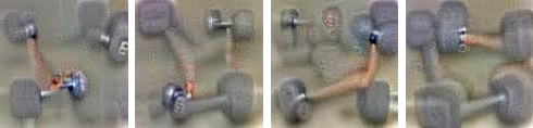
“Here, of course, there are dumbbells, but not a single image of dumbbells seems complete without the presence of muscular roll on it, lifting them,” wrote researchers from Google.

At first glance, this looks strange, but in fact it is not so very different from what people do. If we see a small or blurred object in the picture, we are looking for a hint in his environment in order to understand what may happen there. People obviously argue about the pictures differently, taking advantage of a complex conceptual understanding of the world around them. But in the end, the STS is well recognized by the pictures, because they enjoy all the advantages of the entire context depicted on them, and this is not very different from how people do it.