The book "Machine learning: algorithms for business"

Hi, Habrozhiteli! Marcos Lopez de Prado shares what is usually hidden — the most profitable machine learning algorithms that he used for two decades to manage the large pools of funds of the most demanding investors.

Machine learning changes almost every aspect of our life, MO algorithms perform tasks that until recently trusted only proven experts. In the near future, machine learning will dominate in finance, fortune telling on the tea leaves will be a thing of the past, and investments will no longer be synonymous with gambling.

Take the chance to take part in the “machine revolution” to get to know the first book, which provides a complete and systematic analysis of machine learning methods applied to finance: starting with financial data structures, marking a financial series, weighing the sample, differentiating the time series ... and ending the whole part devoted to the proper backtesting of investment strategies.

Excerpt Understanding risk strategy

15.1. Relevance

Investment strategies are often implemented in terms of positions held until one of two conditions is fulfilled: 1) a condition for exiting a position with profits (taking profits) or 2) a condition for exiting a position with losses (stopping a loss). Even when the strategy does not explicitly declare a loss stop, there is always an implicit stop loss limit at which the investor can no longer finance his position (margin call) or incurs damage caused by an increase in unrealized loss. Since most strategies have (explicitly or implicitly) these two exit conditions, it makes sense to model the distribution of outcomes through a binomial process. This, in turn, will help us understand which combinations of frequency rates, risks, and payouts are uneconomical. The purpose of this chapter is to help you evaluate when a strategy is vulnerable to small changes in any of these dimensions.
')
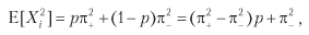
Consider a strategy that produces n equally distributed mutually independent rates per year, where the outcome Xi of the bet i ∈ [1, n] is the profit π> 0 with probability P [Xi = π] = p and loss –π with probability P [Xi = –Π] = 1 - p. You can think of p as the accuracy of a binary classifier, in which an affirmative means a bet on an opportunity, and a negative outcome means an omission of an opportunity: true statements are rewarded, false statements are punished, and negative outcomes (true or false) do not have payments. Since the outcomes of the bets {Xi} i = 1, ..., n are independent, we will calculate the expected moments per bet. The expected profit from one bet is E [Xi] = πp + (–π) (1 - p) = π (2p - 1). Dispersion is 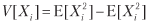where = π2p + (–π) 2 (1 - p) = π2, therefore, V [Xi] = π2 - π2 (2p - 1) 2 = π2 [1– (2p - 1) 2] = 4π2p (1 - p ). For n equally distributed mutually independent rates per year, the average Sharpe ratio (θ) is


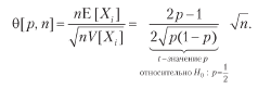
Notice how π balances the above equation, because the payouts are symmetrical. As in the Gaussian case, θ [p, n] can be understood as a solo t-value1. This illustrates the fact that even for small Sharpe ratio can be made high for sufficiently large n. This serves as an economic basis for high-frequency trading, where p may be slightly higher than .5, and an increase in n is the key to successful exchange activity. The Sharpe Ratio is a function of accuracy, and not of correctness, because omission of possibility (negative statement) is not rewarded or punished directly (although too many negative statements can lead to small n, which will reduce the Sharpe ratio to zero).

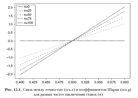
For example, for 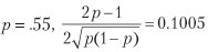and to achieve an average Sharpe ratio of 2, 396 rates per year are required. Listing 15.1 tests this result experimentally. Figure 15.1 shows the Sharpe ratio as a function of accuracy for different frequency rates.

Listing 15.1. Sharpe Ratio as a function of the number of bets

out,p=[],.55 for i in xrange(1000000): rnd=np.random.binomial(n=1,p=p) x=(1 if rnd==1 else -1) out.append(x) print np.mean(out),np.std(out),np.mean(out)/np.std(out)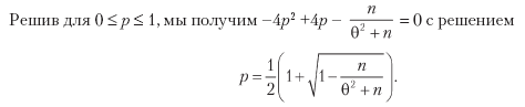 

This equation clearly expresses the trade-off between accuracy (p) and frequency (n) for a given Sharpe ratio (θ). For example, in order to give an average Sharpe coefficient of 2, a strategy that produces only weekly rates (n = 52) will require a fairly high accuracy of p = 0.6336.

15.3. Asymmetrical payouts

Consider a strategy that produces n equally distributed mutually independent rates per year, where the outcome Xi of the bet i ∈ [1, n] is π + with probability P [Xi = π +] = p, and the outcome π– (π– <π + ) happens with probability P [Xi = π_] = 1 - p. The expected profit from one bet is E [Xi] = pπ + + (1 - p) π– = (π + - π–) p + π–. The variance is V [Xi] =, where



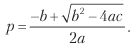
Finally, we can solve the previous equation for 0 ≤ p ≤ 1 and get


Where:
a = (n + θ2) (π + - π–) 2;
b = [2nπ - θ2 (π + - π -)] (π + - π–);


Note: Listing 15.2 tests these symbolic operations using the SymPy Live Python shell running on the Google App Engine cloud service: live.sympy.org .

Listing 15.2. Using the symPy library for symbolic operations

 >>> from sympy import * >>> init_printing(use_unicode=False,wrap_line=False,no_global=True) >>> p,u,d=symbols('pu d') >>> m2=p*u**2+(1-p)*d**2 >>> m1=p*u+(1-p)*d >>> v=m2-m1**2 >>> factor(v) 

The above equation answers the following question: for a given trade rule characterized by the parameters {π–, π +, n}, what is the degree of accuracy p necessary to achieve a Sharpe ratio of θ *? For example, in order to get θ = 2 for n = 260, π– = –.01, π + = .005, we need p = .72. Due to the large number of bets, a very small change in p (from p = .7 to p = .72) advanced the Sharpe ratio from θ = 1.173 to θ = 2. On the other hand, this also tells us that this strategy is vulnerable to small changes in p. Listing 15.3 implements the derivation of the intended accuracy. In fig. 15.2 shows the assumed accuracy as a function of n and π–, where π + = 0.1 and θ * = 1.5. As the threshold π– becomes more negative for a given n, a higher degree p is required to achieve θ * for a given threshold π +. As the number n becomes smaller for a given threshold π–, a higher degree p is required to achieve θ * for a given π +.

Listing 15.3. Calculate Expected Accuracy

 def binHR(sl,pt,freq,tSR): ´´´ 

Given a trade rule characterized by the parameters {sl, pt, freq}, what is the minimum accuracy required to achieve a Sharp coefficient equal to tSR?

1) Inputs
sl: stop loss threshold
pt: profit threshold
freq: number of bids per year
tSR: target annual Sharpe ratio
2) Exit
p: minimum degree of accuracy p required to achieve tSR
´´´
a = (freq + tSR ** 2) * (pt-sl) ** 2
b = (2 * freq * sl-tSR ** 2 * (pt-sl)) * (pt-sl)
c = freq * sl ** 2
p = (- b + (b ** 2–4 * a * c) **. 5) / (2. * a)
return p


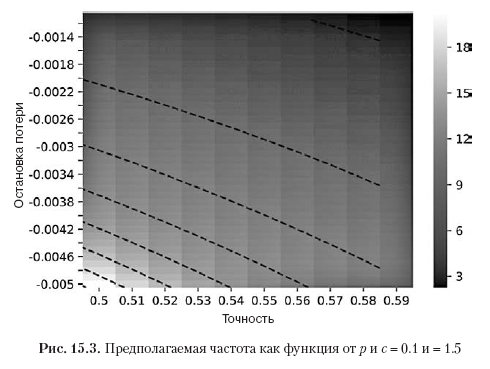
Listing 15.4 solves θ [p, n, π–, π +] for the estimated frequency of betting n. In fig. 15.3 shows the estimated frequency depending on p and π–, where π + = 0.1, and θ * = 1.5. As the threshold π– becomes more negative for a given degree p, a higher number n is required to achieve θ * for a given threshold π +. As for a given threshold π–, the degree p becomes smaller, a higher number n is required, which is necessary to achieve θ * for a given threshold π +.

Listing 15.4. Calculate the estimated frequency of betting

 def binFreq(sl,pt,p,tSR): ´´´ 

Given a trade rule characterized by the parameters {sl, pt, freq}, what number of bids per year is needed to achieve the Sharp tSR with a degree of accuracy p?

Note: radical equation, check for extraneous solution.

1) Inputs
sl: stop loss threshold
pt: profit threshold
p: degree of accuracy p
tSR: target annual Sharpe ratio
2) Exit
freq: the number of required rates per year
´´´
freq = (tSR * (pt-sl)) ** 2 * p * (1-p) / ((pt-sl) * p + sl) ** 2 # possible extraneous
if not np.isclose (binSR (sl, pt, freq, p), tSR): return
return freq



»More information about the book can be found on the publisher's website.
» Table of Contents
» Excerpt

For Habrozhiteley a 25% discount on coupon - Machine Learning

Upon payment of the paper version of the book, an electronic version of the book is sent to the e-mail.