Solving Japanese crosswords with P̶y̶t̶h̶o̶̶n̶ Rust and WebAssembly

How to make a solver (solver) of nonograms in Python, rewrite it in Rust to run directly in a browser via WebAssembly.
Start
About Japanese crosswords (nonograms) on Habré there were already several posts. Example
and one more .
Images are encrypted with numbers to the left of the rows, as well as above the columns. The number of numbers shows how many groups of black (or their own color, for color crossword puzzles) cells are in the corresponding row or column, and the numbers themselves - how many flat cells each of these groups contains (for example, a set of three numbers - 4, 1, and 3 means that there are three groups in this series: the first is from four, the second is from one, the third is from three black cells). In a black-and-white crossword, groups should be separated by at least one empty cell, in color this rule applies only to monochrome groups, and multi-colored groups can be located closely (empty cells can be along the edges of the rows). It is necessary to determine the placement of groups of cells.
One of the most common points of view is that only correct ones can be called “correct” crossword puzzles. Usually, this is how a solution method is called, in which the dependencies between different rows and / or columns are not taken into account. In other words, a solution is a sequence of independent decisions of individual rows or columns, until all cells are painted over (for more details about the algorithm, see below). For example, only such nonograms can be found at http://nonograms.org/ ( http://nonograms.ru/ ). Nonograms from this site have already been cited as an example in the article Solving colored Japanese crosswords with the speed of light . For comparison and verification purposes, support for downloading and parsing crosswords from this site has also been added to my solver (thanks to KyberPrizrak for permission to use materials from his site).
However, it is possible to extend the concept of nonograms to a more general problem, when the usual “logical” method leads to a dead end. In such cases, to solve, you have to make an assumption about the color of a cell and then, having proved that this color leads to a contradiction, mark the opposite color for this cell. The sequence of such steps can (if there is enough patience) give us all the solutions. About solving such a more general case of crossword puzzles and will be mainly this article.
Python
About a year and a half ago, I accidentally stumbled upon an article in which I was told how to solve one line (as it turned out later, the method was rather slow).
When I implemented this method in Python (my main working language) and added a sequential update of all lines, I saw that all of this was not solved very quickly. After studying the materiel, it turned out that there are a lot of works and implementations on this topic that offer different approaches for this task.
It seemed to me that the most extensive work on the analysis of various implementations of solvers was done by Jan Wolter, publishing on his website (which, as far as I know, remains the largest public repository of nonograms on the Internet) a detailed study containing a huge amount of information and links that can help creating your solver.
Studying numerous sources (will be at the end of the article), I gradually improved the speed and functionality of my solver. As a result, I was dragged out and I was engaged in the implementation, refactoring, debugging algorithms for about 10 months in the working time.
Basic algorithms
The resulting solver can be represented in the form of four levels of solution:
( line ) linear solver: at the input, a line of cells and a line of description (clues), at the output - a partially solved line. In the python solution, I implemented 4 different algorithms (3 of them are adapted for color crosswords). The fastest was the BguSolver algorithm, named after the original source . This is a very effective and actually standard method for solving nonogram strings using dynamic programming. Pseudocode of this method can be found for example in this article .
( propagation ) we add all the rows and columns to the queue, we pass through it with a linear solver, when we receive new information when we solve the row (column) we update the queue, respectively, with new columns (rows). We continue until the queue is empty.
Example and CodeWe take the next task to solve the queue. Let it be an empty (unresolved) string of length 7 (we denote it as
???????) with a description of the blocks[2, 3]. Linear solver will issue a partially resolved string?X??XX?whereXis a filled cell. When updating the row, we see that the columns with numbers 1, 4, 5 have changed (indexing starts from 0). This means that new information has appeared in the indicated columns and they can be given back to the “linear” solver. We add these columns to the task queue with an increased priority (in order to give them to the linear solver as follows).def propagation(board): line_jobs = PriorityDict() for row_index in range(board.height): new_job = (False, row_index) line_jobs[new_job] = 0 for column_index in range(board.width): new_job = (True, column_index) line_jobs[new_job] = 0 for (is_column, index), priority in line_jobs.sorted_iter(): new_jobs = solve_and_update(board, index, is_column) for new_job in new_jobs: # upgrade priority new_priority = priority - 1 line_jobs[new_job] = new_priority def solve_and_update(board, index, is_column): if is_column: row_desc = board.columns_descriptions[index] row = tuple(board.get_column(index)) else: row_desc = board.rows_descriptions[index] row = tuple(board.get_row(index)) updated = line_solver(row_desc, row) if row != updated: for i, (pre, post) in enumerate(zip(row, updated)): if _is_pixel_updated(pre, post): yield (not is_column, i) if is_column: board.set_column(index, updated) else: board.set_row(index, updated)
( probing ) for each unresolved cell we search through all the color options and try propagation with this new information. If we get a contradiction, we throw this color out of the color options for the cell and try to benefit from it again with the help of propagation. If it is solved to the end, we add the solution to the list of solutions, but continue to experiment with other colors (there may be several solutions). If we come to a situation where it is impossible to solve further, we simply ignore and repeat the procedure with a different color / cell.
CodeReturns True if a conflict was obtained as a result of the probe.
def probe(self, cell_state): board = self.board pos, assumption = cell_state.position, cell_state.color # already solved if board.is_cell_solved(pos): return False if assumption not in board.cell_colors(pos): LOG.warning("The probe is useless: color '%s' already unset", assumption) return False save = board.make_snapshot() try: board.set_color(cell_state) propagation( board, row_indexes=(cell_state.row_index,), column_indexes=(cell_state.column_index,)) except NonogramError: LOG.debug('Contradiction', exc_info=True) # rollback solved cells board.restore(save) else: if board.is_solved_full: self._add_solution() board.restore(save) return False LOG.info('Found contradiction at (%i, %i)', *pos) try: board.unset_color(cell_state) except ValueError as ex: raise NonogramError(str(ex)) propagation( board, row_indexes=(pos.row_index,), column_indexes=(pos.column_index,)) return True
( backtracking ) if, when probing, we do not ignore the partially solved puzzle, but continue to recursively call the same procedure, we will get backtracking (in other words, a complete detour into the depth of the potential decision tree). Here begins to play a large role, which cell will be selected as the next expansion of the potential solution. A good study on this topic is in this publication .
CodeMy backtracking is pretty messy, but these two functions roughly describe what happens during a recursive search.
def search(self, search_directions, path=()): """ Return False if the given path is a dead end (no solutions can be found) """ board = self.board depth = len(path) save = board.make_snapshot() try: while search_directions: state = search_directions.popleft() assumption, pos = state.color, state.position cell_colors = board.cell_colors(pos) if assumption not in cell_colors: LOG.warning("The assumption '%s' is already expired. " "Possible colors for %s are %s", assumption, pos, cell_colors) continue if len(cell_colors) == 1: LOG.warning('Only one color for cell %r left: %s. Solve it unconditionally', pos, assumption) try: self._solve_without_search() except NonogramError: LOG.warning( "The last possible color '%s' for the cell '%s' " "lead to the contradiction. " "The path %s is invalid", assumption, pos, path) return False if board.is_solved_full: self._add_solution() LOG.warning( "The only color '%s' for the cell '%s' lead to full solution. " "No need to traverse the path %s anymore", assumption, pos, path) return True continue rate = board.solution_rate guess_save = board.make_snapshot() try: LOG.warning('Trying state: %s (depth=%d, rate=%.4f, previous=%s)', state, depth, rate, path) success = self._try_state(state, path) finally: board.restore(guess_save) if not success: try: LOG.warning( "Unset the color %s for cell '%s'. Solve it unconditionally", assumption, pos) board.unset_color(state) self._solve_without_search() except ValueError: LOG.warning( "The last possible color '%s' for the cell '%s' " "lead to the contradiction. " "The whole branch (depth=%d) is invalid. ", assumption, pos, depth) return False if board.is_solved_full: self._add_solution() LOG.warning( "The negation of color '%s' for the cell '%s' lead to full solution. " "No need to traverse the path %s anymore", assumption, pos, path) return True finally: # do not restore the solved cells on a root path - they are really solved! if path: board.restore(save) return True def _try_state(self, state, path): board = self.board full_path = path + (state,) probe_jobs = self._get_all_unsolved_jobs(board) try: # update with more prioritized cells for new_job, priority in self._set_guess(state): probe_jobs[new_job] = priority __, best_candidates = self._solve_jobs(probe_jobs) except NonogramError as ex: LOG.warning('Dead end found (%s): %s', full_path[-1], str(ex)) return False rate = board.solution_rate LOG.info('Reached rate %.4f on %s path', rate, full_path) if rate == 1: return True cells_left = round((1 - rate) * board.width * board.height) LOG.info('Unsolved cells left: %d', cells_left) if best_candidates: return self.search(best_candidates, path=full_path) return True
So, we begin to solve our crossword puzzle from the second level (the first one is suitable only for a degenerate case, when there is only one row or column in the whole crossword puzzle) and gradually move up the levels. As you might guess, each level several times causes the underlying level, so for an effective solution it is extremely necessary to have fast first and second levels, which can be called millions of times for complex puzzles.
At this stage it turns out (quite expectedly) that python is not at all the tool that is suitable for maximum performance in such a CPU-intensive task: all the calculations in it are extremely inefficient compared to lower-level languages. For example, the most algorithmically close BGU-solver (in Java) was 7–17 (sometimes up to 27) times faster on a variety of tasks.
         pynogram_my BGU_my speedup
 Dancer 0.976 0.141 6.921986
 Cat 1.064 0.110 9.672727
 Skid 1.084 0.101 10.732673
 Bucks 1.116 0.118 9.457627
 Edge 1.208 0.094 12.851064
 Smoke 1.464 0.120 12.200000
 Knot 1.332 0.140 9.514286
 Swing 1.784 0.138 12.927536
 Mum 2.108 0.147 14.340136
 DiCap 2.076 0.176 11.795455
 Tragic 2.368 0.265 8.935849
 Merka 2.084 0.196 10.632653
 Petro 2.948 0.219 13.461187
 M & M 3.588 0.375 9.568000
 Signed 4.068 0.242 16.809917
 Light 3.848 0.488 7.885246
 Forever 111.000 13.570 8.179808
 Center 5.700 0.327 17.431193
 Hot 3.150 0.278 11.330935
 Karate 2.500 0.219 11.415525
 9-Dom 510.000 70.416 7.242672
 Flag 149.000 5.628 26.474769
 Lion 71.000 2.895 24.525043
 Marley 12.108 4.405 2.748695
 Thing 321,000 46.166 6.953169
 Nature inf 433.138 inf
 Sierp inf inf NaN
 Gettys inf inf NaN
The measurements were taken on my machine, the puzzles are taken from the standard set, which Jan Wolter used in his comparison
And this is already after I started using PyPy, and on standard CPython the calculation time was 4-5 times higher than on PyPy! We can say that the performance of a similar Java solver turned out to be higher than CPython code by 28-85 times.
Attempts to improve the performance of my solver with the help of profiling (cProfile, SnakeViz, line_profiler) led to some acceleration, but they certainly didn’t give a supernatural result.
Results :
+ Solver can solve all puzzles from https://webpbn.com , http://nonograms.org and its own (ini-based) format
+ solves black-and-white and color nonograms with any number of colors (the maximum number of colors that was encountered is 10)
+ Solves puzzles with missing block sizes (blotted). An example of such a puzzle .
+ can render puzzles to the console / to the curses window / to the browser (when installing the additional option pynogram-web ). For all modes, viewing the progress of the solution in real time is supported.
- slow calculations (in comparison with the implementations described in the article-comparison of solvers, see table ).
- ineffective backtracking: some puzzles can be solved for hours (when the decision tree is very large).
Rusty
Earlier this year, I began to study Rust. I started, as usual, with The Book , I learned about WASM, I went through the proposed tutorial . However, I wanted some real task in which the strengths of the language could be acted upon (first of all, its super-performance), and not examples invented by someone. So I went back to the nonograms. But now I already had a working version of all the algorithms in Python, it remains “only” to rewrite.
From the very beginning, the good news was waiting for me: it turned out that Rust, with its type system, perfectly describes the data structures for my task. For example, one of the basic matches BinaryColor + BinaryBlock / MultiColor + ColoredBlock allows you to permanently separate black and white and colored nonograms. If somewhere in the code we try to solve a color string using ordinary binary description blocks, we get a compilation error about the type mismatch.
pub trait Color { fn blank() -> Self; fn is_solved(&self) -> bool; fn solution_rate(&self) -> f64; fn is_updated_with(&self, new: &Self) -> Result<bool, String>; fn variants(&self) -> Vec<Self>; fn as_color_id(&self) -> Option<ColorId>; fn from_color_ids(ids: &[ColorId]) -> Self; } pub trait Block { type Color: Color; fn from_str_and_color(s: &str, color: Option<ColorId>) -> Self { let size = s.parse::<usize>().expect("Non-integer block size given"); Self::from_size_and_color(size, color) } fn from_size_and_color(size: usize, color: Option<ColorId>) -> Self; fn size(&self) -> usize; fn color(&self) -> Self::Color; } #[derive(Debug, PartialEq, Eq, Hash, Clone)] pub struct Description<T: Block> where T: Block, { pub vec: Vec<T>, } // for black-and-white puzzles #[derive(Debug, PartialEq, Eq, Hash, Copy, Clone, PartialOrd)] pub enum BinaryColor { Undefined, White, Black, BlackOrWhite, } impl Color for BinaryColor { // omitted } #[derive(Debug, PartialEq, Eq, Hash, Default, Clone)] pub struct BinaryBlock(pub usize); impl Block for BinaryBlock { type Color = BinaryColor; // omitted } // for multicolor puzzles #[derive(Debug, PartialEq, Eq, Hash, Default, Copy, Clone, PartialOrd, Ord)] pub struct MultiColor(pub ColorId); impl Color for MultiColor { // omitted } #[derive(Debug, PartialEq, Eq, Hash, Default, Clone)] pub struct ColoredBlock { size: usize, color: ColorId, } impl Block for ColoredBlock { type Color = MultiColor; // omitted } When migrating the code, some moments clearly indicated that a statically typed language, such as Rust (or, for example, C ++), is more suitable for this task. More precisely, generics and traits describe the subject area better than class hierarchies. So in the Python code, I had two classes for a linear BguSolver , BguSolver and BguColoredSolver which decided, respectively, the black-and-white line and the color line. In the Rust code, I still have a single generic structure struct DynamicSolver<B: Block, S = <B as Block>::Color> , which can solve both types of tasks, depending on the type transferred during creation ( DynamicSolver<BinaryBlock>, DynamicSolver<ColoredBlock> ). This, of course, does not mean that something similar cannot be done in Python, just in Rust the type system explicitly indicated to me that if you do not go this way, you will have to write a ton of duplicate code.
In addition, anyone who tried to write on Rust undoubtedly noticed the effect of "trusting" the compiler, when the process of writing code reduces to the following pseudo-meta-algorithm:
 write_initial_code
 while (compiler_hints = $ (cargo check))! = 0;  do
     fix_errors (compiler_hints)
 end
When the compiler stops issuing errors and warnings, your code will be coordinated with the type system and borrow checker and you will warn in advance of a heap of potential bugs (of course, subject to careful design of data types).
I will give a couple of examples of functions that show how concise Rust code can be (compared to Python analogues).
List the unresolved "neighbors" for a given point (x, y)
def unsolved_neighbours(self, position): for pos in self.neighbours(position): if not self.is_cell_solved(*pos): yield pos fn unsolved_neighbours(&self, point: &Point) -> impl Iterator<Item = Point> + '_ { self.neighbours(&point) .into_iter() .filter(move |n| !self.cell(n).is_solved()) } For a set of blocks describing a single line, give partial amounts (taking into account the mandatory intervals between blocks). The resulting indices will indicate the minimum position where the block can end (this information is used further for a linear solver).
For example, for such a set of blocks [2, 3, 1] we have the output [2, 6, 8] , which means that the first block can be shifted to the left as much as possible so that its right edge occupies the 2nd cell, similarly for the rest blocks:
             1 2 3 4 5 6 7 8 9
             _ _ _ _ _ _ _ _ _
      2 3 1 | _ | _ | _ | _ | _ | _ | _ | _ | _ |
               ^ ^ ^
               |  |  |
 end of block 1 |  |  |
 end of block 2 -------- |
 end of block 3 ------------
@expand_generator def partial_sums(blocks): if not blocks: return sum_so_far = blocks[0] yield sum_so_far for block in blocks[1:]: sum_so_far += block + 1 yield sum_so_far fn partial_sums(desc: &[Self]) -> Vec<usize> { desc.iter() .scan(None, |prev, block| { let current = if let Some(ref prev_size) = prev { prev_size + block.0 + 1 } else { block.0 }; *prev = Some(current); *prev }) .collect() } When porting, I made a few changes.
- the core of the solver (algorithms) has undergone minor changes (primarily to support generic types for cells and blocks)
- left the only (fastest) algorithm for linear solver
- instead of ini format introduced a slightly modified TOML format
- did not add support for blotted crosswords, because, strictly speaking, this is a different class of tasks
left the only way out - just to the console, but now the colored cells in the console are drawn really colored (thanks to this crete )
like this
Useful tools
- clippy - a standard static analyzer, which sometimes can even give tips that slightly increase code performance
- valgrind is a tool for dynamic analysis of applications. I used it as a profiler to search for bottlenecks (
valrgind --tool=callgrind) and especially voracious parts of the code (valrgind --tool=massif). Tip: set [profile.release] debug = true in Cargo.toml before running the profiler. This will leave the debug characters in the executable file. - kcachegrind for viewing callgrind files. A very useful tool for finding the most problematic places in terms of performance.
Performance
That for the sake of what was being started and rewriting Rust. We take crosswords from the already mentioned comparison table and run them through the best solvers described in the original article. Results and description of the runs here . We take the resulting file and build a couple of graphs on it. Since the solution time varies from milliseconds to tens of minutes, the graph is executed with a logarithmic scale.
import pandas as pd import numpy as np import matplotlib.pyplot as plt %matplotlib inline # strip the spaces df = pd.read_csv('perf.csv', skipinitialspace=True) df.columns = df.columns.str.strip() df['name'] = df['name'].str.strip() # convert to numeric df = df.replace('\+\ *', np.inf, regex=True) ALL_SOLVERS = list(df.columns[3:]) df.loc[:,ALL_SOLVERS] = df.loc[:,ALL_SOLVERS].apply(pd.to_numeric) # it cannot be a total zero df = df.replace(0, 0.001) #df.set_index('name', inplace=True) SURVEY_SOLVERS = [s for s in ALL_SOLVERS if not s.endswith('_my')] MY_MACHINE_SOLVERS = [s for s in ALL_SOLVERS if s.endswith('_my') and s[:-3] in SURVEY_SOLVERS] MY_SOLVERS = [s for s in ALL_SOLVERS if s.endswith('_my') and s[:-3] not in SURVEY_SOLVERS] bar_width = 0.17 df_compare = df.replace(np.inf, 10000, regex=True) plt.rcParams.update({'font.size': 20}) def compare(first, others): bars = [first] + list(others) index = np.arange(len(df)) fig, ax = plt.subplots(figsize=(30,10)) df_compare.sort_values(first, inplace=True) for i, column in enumerate(bars): ax.bar(index + bar_width*i, df_compare[column], bar_width, label=column[:-3]) ax.set_xlabel("puzzles") ax.set_ylabel("Time, s (log)") ax.set_title("Compare '{}' with others (lower is better)".format(first[:-3])) ax.set_xticks(index + bar_width / 2) ax.set_xticklabels("#" + df_compare['ID'].astype(str) + ": " + df_compare['name'].astype(str)) ax.legend() plt.yscale('log') plt.xticks(rotation=90) plt.show() fig.savefig(first[:-3] + '.png', bbox_inches='tight') for my in MY_SOLVERS: compare(my, MY_MACHINE_SOLVERS) compare(MY_SOLVERS[0], MY_SOLVERS[1:]) python solver
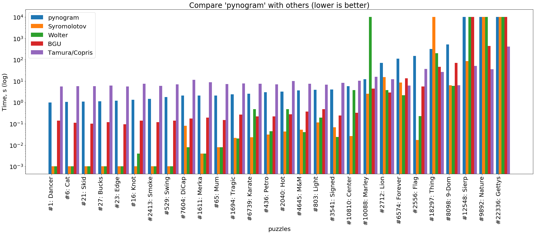
(the picture is clickable )
We see that the pynogram here is the slowest of all represented solvers. The only exception to this rule is the Tamura / Copris solver, based on the SAT, which solves the simplest puzzles (the left part of the graph) longer than ours. However, such is the peculiarity of SAT-solvers: they are designed for super complex crosswords, in which an ordinary solver is stuck in backtracking for a long time. This is clearly visible on the right side of the chart, where Tamura / Copris solves the most difficult puzzles tens and hundreds of times faster than any other.
rustler
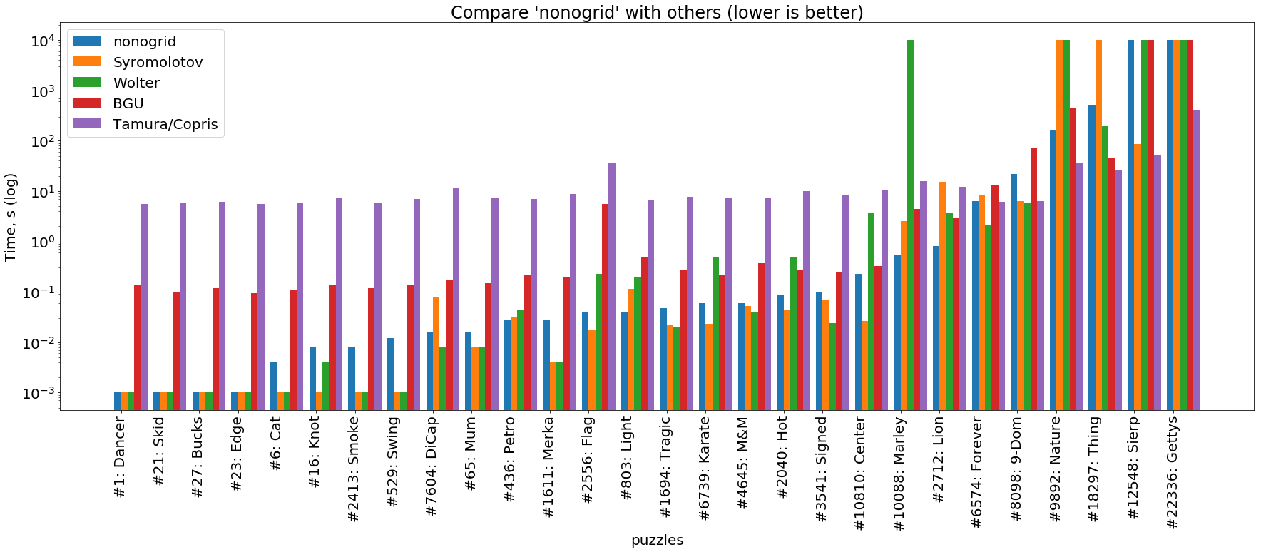
(the picture is clickable )
This graph shows that nonogrid copes with simple tasks as well or slightly worse than high-performance solvers written in C and C ++ ( Wolter and Syromolotov ). With the complication of tasks, our solver roughly repeats the trajectory of a BGU solver (Java), but almost always advances it by an order of magnitude. On the most difficult tasks, Tamura / Copris is always ahead of everyone.
rust vs python
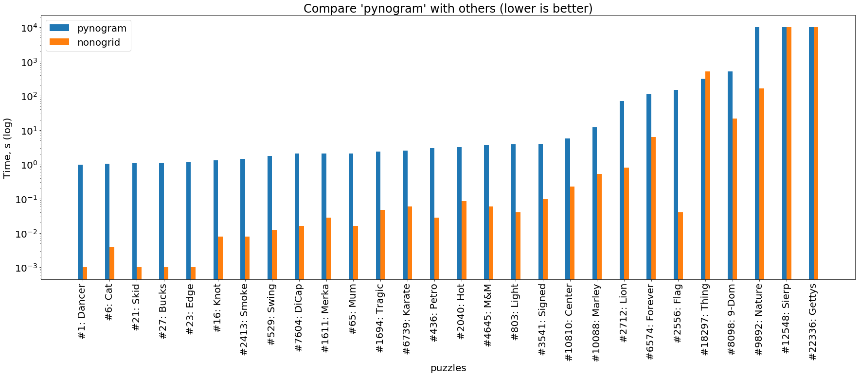
(the picture is clickable )
Well, finally, a comparison of our two solvers, described here. It can be seen that the Rust-solver is almost always ahead of the Piton solver by 1–3 orders of magnitude.
Results :
+ Solver can solve all puzzles from https://webpbn.com (except blotted - with partially hidden block sizes), http://nonograms.org and its own (TOML-based) format
+ solves black and white and color nonograms with any number of colors
+ can render puzzles to console (color c with webpbn.com draws truly color)
+ works quickly (in comparison with the implementations described in the article-comparison of solvers, see table).
- backtracking remained inefficient, as in the Python-solution: some puzzles (for example , such a harmless 20x20 ) can be solved for hours (when the decision tree is very large). Perhaps instead of backtracking, you should use the SAT-solvers already mentioned in the habr . True, the only SAT-solver I found on Rust at first glance seems to be underdeveloped and abandoned.
WebAssembly
So, rewriting the code to Rust has borne fruit: the solver has become much faster. However, Rust offers us another incredibly cool feature: compiling to WebAssembly and the ability to run your code directly in the browser.
To implement this feature, there is a special tool for Rust, which provides the necessary binders and generates a boilerplate for you to run Rust functions painlessly in the JS code - this wasm-pack (+ wasm-bindgen ). Most of the work with it and other important tools is already described in the Rust and WebAssembly tutorial . However, there are a couple of things that I had to figure out on my own:
reading gives the impression that the tutorial is primarily written for a JS developer who wants to speed up his code with Rust. Or at least for someone who is familiar with npm . For me, as a person far from the front-end, it was a surprise to discover that even the standard book example does not want to work with a third-party web server different from
npm run start.Fortunately, the wasm-pack has a mode that allows you to generate a regular JS code (which is not an npm module).
wasm-pack build --target no-modules --no-typescriptwill yield only two files at the output: project-name.wasm - Rust-code binary compiled in WebAssembly and project-name.js . You can add the latest file to any HTML<script src="project-name.js"></script>page and use WASM functions without bothering with npm, webpack, ES6, modules and other joys of a modern JS developer. Theno-modulesmode is ideal for non-frontenders during the development of a WASM application, as well as for examples and demonstrations, because it does not require any additional frontend infrastructure.WemAssembly is good for tasks that are too heavy for javascript. First of all, these are tasks that perform many calculations. And if so, this task can be performed for a long time even with WebAssembly and thus violate the asynchronous principle of the modern web. I'm talking about all sorts of Warning: Unresponsive script , which I happened to observe while working my solver. To solve this problem, you can use the mechanism of Web worker . In this case, the scheme of work with "heavy" WASM-functions may look like this:
- from the main script of the event (for example, clicking on a button) send a message to the worker with the task to start a heavy function.
- , .
- - ()
WASM- JS, WASM . - ( ), HashMap , . ( JS) , / .
, Mutex , thread-safe. smart- . thread-safe Rc Arc RefCell RwLock . : 30%. --features=threaded thread-safe , WASM-.
| id | non-thread-safe | thread-safe | web-interface |
|---|---|---|---|
| 6574 | 5.4 | 7.4 | 9.2 |
| 8098 | 21.5 | 28.4 | 29.9 |
, - 40..70% , , (32..37%) thread-safe ( cargo build --release --features=threaded ).
Firefox 67.0 Chromium 74.0.
WASM- ( ). https://webpbn.com/ http://www.nonograms.org/
Todo
"" /, / .
, . "" , , . .
( , 3600 ). WASM , ( , (!) , , WASM). , , - , nonogrid .
. : , , WASM . , ( ) , JS , .
JS. backtrace, .
( TOML- )
Results
, (, , etc).
Rust 1-3 PyPy 1.5-2 ( ).
Python Rust , Python (, , comprehensions), Rust-.
Rust WebAssembly . Rust , WASM, ( 1.5 ).
')
Source: https://habr.com/ru/post/454586/
All Articles