Sounding the past. A guide for historians to convert data into sound
I'm sick of looking at the past. There are many guidelines for recreating the appearance of historical artifacts, but often we forget that this is a creative act. Perhaps we are too attached to our screens, we attach too much importance to our appearance. Let's try to hear something from the past instead.
The rich literature on archeoacoustics and sound landscapes helps to recreate the sound of a place as it was (for example, see the Virtual Cathedral of St. Paul or the work of Jeff Weitch on ancient Ostia ). But it is interesting to me to “voice” the data itself. I want to define the syntax for representing data in the form of sound, so that these algorithms can be used in historical science. Drucker said the famous phrase that “data” is not really what is given, but rather what is captured, transformed, that is, 'capta'. When dubbing data, I literally reproduce the past in the present. Therefore, the assumptions and transformations of this data come to the fore. The resulting sounds are “deformed performance”, which makes you hear the modern layers of history in a new way.
I want to hear the meaning of the past, but I know that this is impossible. However, when I hear an instrument, I can physically present a musician; on the echoes and resonances can distinguish the physical space. I feel the bass, can move in rhythm. Music covers my body, all imagination. Associations with previously heard sounds, music, and tones create a deep temporal experience, a system of embodied relationships between me and the past. Visuality? We have so long been visual representations of the past, that these grammars almost lost their artistic expressiveness and performative aspect.
In this lesson you will learn how to create some noise from historical data. The value of this noise, well ... depends on you. Partially the point is to make your data unfamiliar again. Translating, recoding, restoring them, we begin to see the data elements that remained invisible by visual examination. This deformation is consistent with the arguments made, for example, by Mark Sample about the deformation of society or Bethany Nowowiski about the "resistance of materials" . Voiceover leads us from data to the “capt”, from social sciences to art, from glitch to aesthetics . Let's see what it looks like.
')
In this lesson, I will discuss three ways to generate sound or music from your data.
We will first use the free and open Musicalgorithms system developed by Jonathan Middleton. In it we will get acquainted with key problems and terms. Then take a small Python library to “translate” data onto an 88-key keyboard and bring some creativity to the work. Finally, load the data into Sonic Pi's real-time audio and music processing software, for which many tutorials and reference resources are published.
You will see how working with sounds moves us from a simple visualization into a really effective environment.
Sonification is a method of translating certain aspects of data into audio signals. In general, a method can be called “sounding” if it satisfies certain conditions. These include reproducibility (other researchers can process the same data in the same way and get the same results) and what can be called “intelligibility” or “intelligibility”, that is, when significant elements of the source data are systematically reflected in the resulting sound (see Hermann, 2008 ). Mark Last and Anna Usyskina (2015) described a series of experiments to determine which analytical tasks can be performed on dubbing data. Their experimental results showed that even untrained listeners (without formal learning to music) can discern the data aurally and make useful conclusions. They found that listeners are able to perform common data mining tasks by ear, such as classification and clustering (in their experiments they broadcast basic scientific data on a scale of Western music).
Last and Usyskina focused on time series. According to their conclusions, time-series data is particularly well-suited for dubbing, since there are natural parallels here. The music is consistent, it has a duration, and it develops over time; likewise with the data of time series ( Last, Usyskina 2015: p. 424 ). It remains to compare the data with the corresponding audio outputs. To combine aspects of data from different auditory measurements, such as height, variation form, and spacing (onset), the parameter mapping method is used in many applications. The problem with this approach is that if there is no temporal relationship between the source data points (or, rather, a non-linear relationship), the resulting sound can be “entangled” ( 2015: 422 ).
Listening to the sound, a person fills the moments of silence with his expectations. Consider a video where mp3 is converted to MIDI and back to mp3; the music is “flattened”, so that all the sound information is reproduced by one tool (the effect is similar to saving a web page as .txt, opening it in Word, and then re-saving it in .html format). All sounds (including vocals) are converted to the corresponding note values, and then back to mp3.
This is noise, but the meaning can be caught:
What's going on here? If this song was known to you, you probably understood the real “words”. But there are no words in the song! If you have not heard it before, then it sounds like a meaningless cacophony (more examples on Andy Bayo site). This effect is sometimes called “sound hallucination” (auditory hallucination). The example shows how in any data representation we can hear / see what, strictly speaking, no. We fill the void with our own expectations.
What does this mean for the story? If we voice our data and begin to hear patterns in sound or weird outliers, then our cultural expectations about music (memories of similar fragments of music heard in certain contexts) will color our interpretation. I would say that this is true for all perceptions of the past, but sounding is quite different from standard methods, so this self-awareness helps identify or express certain critical patterns in (data about) the past.
Consider three tools for dubbing data and note how the choice of instrument affects the result, and how to solve this problem by rethinking the data in another tool. In the end, sounding is not more objective than visualization, so the researcher must be ready to justify his choice and make this choice transparent and reproducible. (So that no one would think that sounding and algorithmically generated music is something new, I send an interested reader to Hedges, 1978 ).
Each section contains a conceptual introduction, and then a step-by-step guide using samples of archaeological or historical data.
There is a wide range of tools for voicing data. For example, packages for the popular statistical R environment , such as playitbyR and AudiolyzR . But the first one is not supported in the current version of R (the last update was several years ago), and in order to make the second one work properly, a serious configuration of additional software is required.
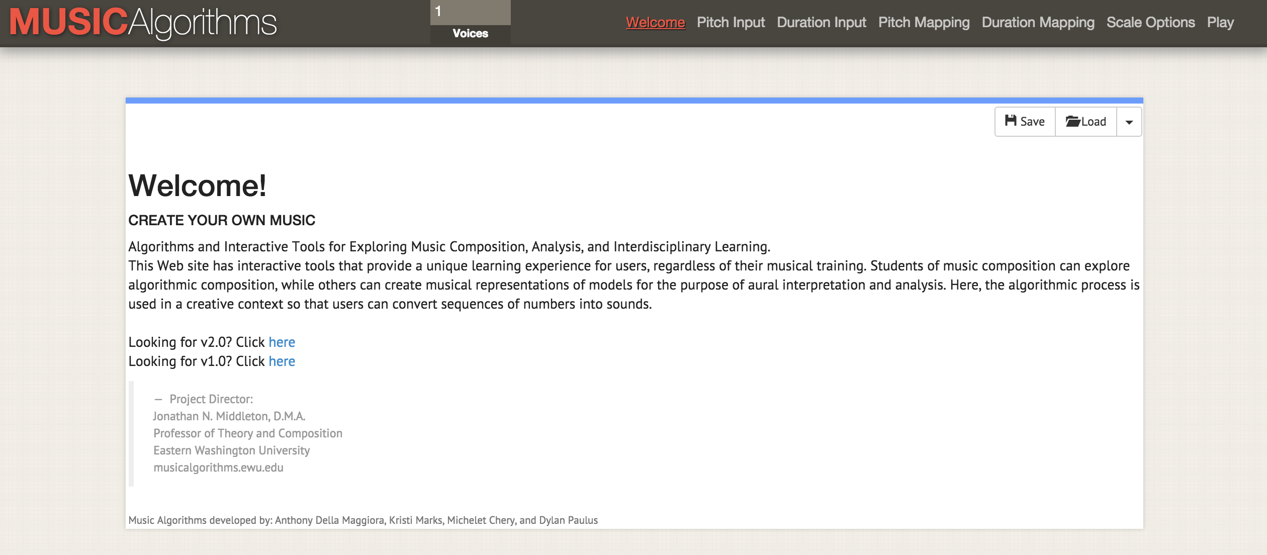
In contrast, the Musical algorithms website is quite simple to use, it has been running for more than ten years. Although the source code has not been published, it is a long-term research project on computational music from Jonathan Middleton. It is currently in the third major version (previous iterations are available on the Internet). We start with Musicalalgorithms, because it allows us to quickly load and tune our data for the release of the presentation as MIDI files. Before you begin, be sure to select the third version .
Site Musicalgorithms as of February 2, 2016
Musicalgorithms produces a series of transformations with data. In the example below (by default on the site), there is only one line of data, although it looks like several lines. This pattern consists of fields, separated by commas, which are internally separated by spaces.
These figures represent the source data and their conversion. Sharing a file allows another researcher to repeat the work or continue processing with other tools. If you start from the beginning, then you need only the source data below (a list of data points):
For us, the key is the 'areaPitch1' field with input data, which are separated by spaces. Other fields will be filled in during work with various Musicalgorithms settings. In the above data (for example, 24 72 12 84, etc.), the values represent the initial calculations of the number of inscriptions in British cities along the Roman road (later we will practice with other data).

After loading data in the top menu bar, you can select various operations. In the screenshot, hovering the mouse over information displays an explanation of what happens when you select a division operation to scale the data to the selected range of notes.
Now when viewing various tabs in the interface (duration, height translation, duration translation, scale parameters) various transformations are available. In the “pitch mapping”, there are a number of mathematical options for translating data to the full 88-key piano keyboard (in linear broadcasting, the average value is transmitted to the average C, that is, 40). You can also choose the type of scale: minor or major and so on. At this stage, after selecting various transformations, it is necessary to save the text file. On the File → Play tab, you can upload a midi file. Your audio program should be able to play midi by default (often the notes of the piano are used by default). More complex midi tools are assigned in mixer programs, such as GarageBand (Mac) or LMMS (Windows, Mac, Linux). However, the use of GarageBand and LMMS is beyond the scope of this guide: a video tutorial on LMMS is available here , and GarageBand tutorials are full on the Internet. For example, a great guide to Lynda.com.
It happens that for the same points there are several columns of data. Say, in our example from Britain, we want to voice also a calculation on the types of ceramics for the same cities. Then you can reload the next row of data, transform and match, and create another MIDI file. Since GarageBand and LMMS allow you to overlay voices, creating complex music sequences is available.
Screenshot GarageBand, where midi-files are voiced themes from the diary of John Adams. In the GarageBand (and LMMS) interface, each midi-file is dragged with the mouse to the appropriate place. The toolkit of each midi file (i.e. tracks) is selected in the GarageBand menu. Track labels are changed to reflect keywords in each topic. The green area on the right is a visualization of notes on each track. You can watch this interface in action and listen to music here.
What transformations to use? If you have two columns of data, these are two voices. Perhaps in our hypothetical data it makes sense to reproduce the first voice loudly as the main one: in the end, the inscriptions in a certain way “speak” with us (Roman inscriptions literally refer to passersby: “O you passing by ...”). And pottery, perhaps, is a more modest artifact, which can be compared with the lower end of the scale or increase the duration of notes, reflecting its omnipresence among representatives of different classes in this region.
There is no single “right” way to translate data to sound , at least not yet. But even in this simple example, we see how shades of meaning and interpretation appear in the data and their perception.
What about time? Historical data often has a specific date reference. Thus, it is necessary to take into account the time interval between two data points. This is where our next tool becomes useful if the data points correspond to each other in space. We begin to move from sound (data points) to music (the relationship between the points).
In the first column of the data set - the number of Roman coins and the amount of other materials from the same cities. Info taken from the British Museum's Portable Antiquities Scheme. Processing this data may reveal some aspects of the economic situation along Watling Street, the main route through Roman Britain. Data points are geographically located from northwest to southeast; so as we play the sound, we hear movement in space. Each note represents each stop on the way.
So, we voiced one column of data! Click 'Save', then 'Save CSV'.
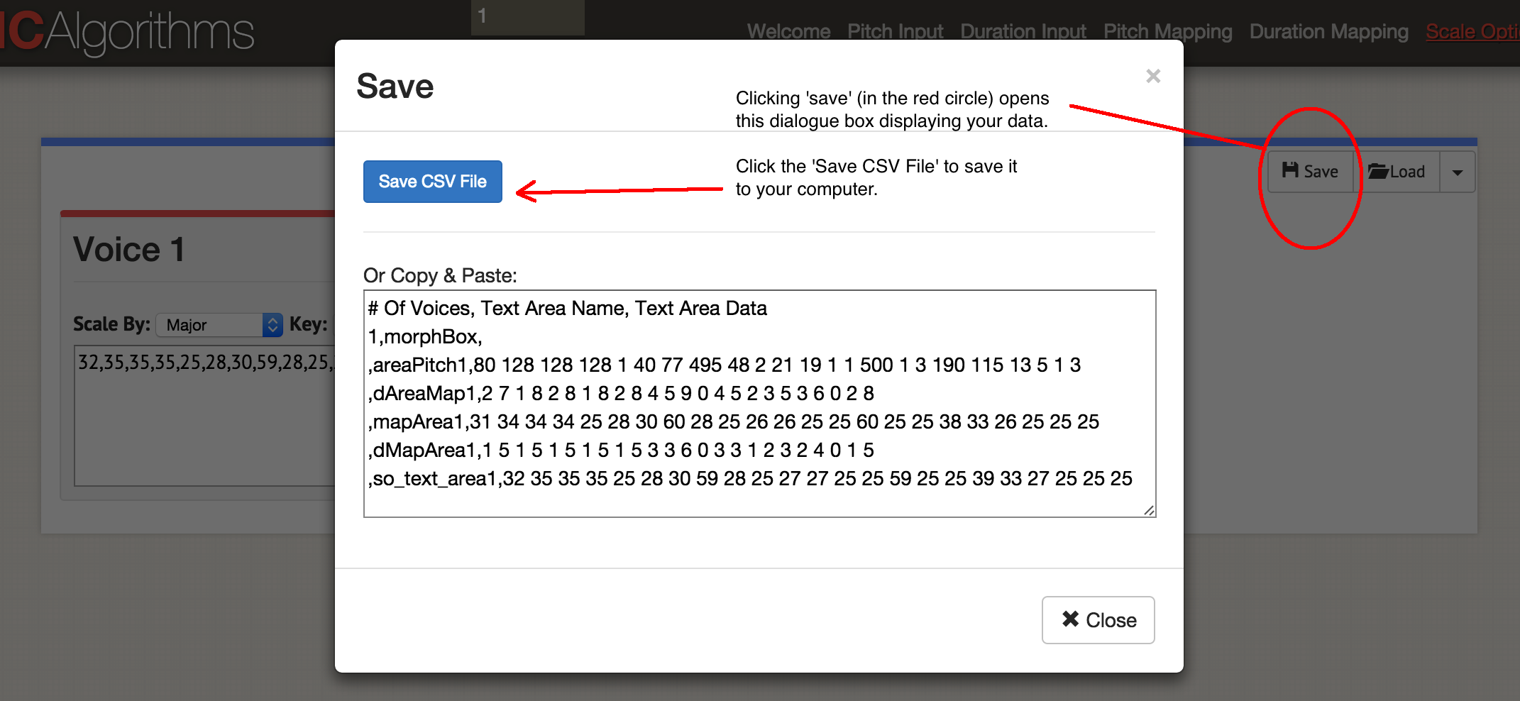
Dialog box 'Save'
You will get something like this:
The original data remained in the 'areaPitch1' field, and then the mappings follow. The site allows you to generate in one MIDI file up to four voices simultaneously. Depending on which instruments you wish to use later, you can choose to generate one MIDI file at a time. Let's start the music: click 'Play'. Here you choose the tempo and instrument. You can listen to your data in the browser or save it as a MIDI file with the blue 'Save MIDI file' button.
Let's go back to the beginning and load both data columns into this template:
Here we are on the page with the 'pitch input' parameters. At the top of the window, enter two voices, now on any page with parameters two windows open for two voices. As before, we load the data in CSV format, but the file needs to be formatted so that the values of 'areaPitch1' and 'areaPitch2' are indicated there. Data for the first voice will appear on the left, and the second - on the right.
If we have a few voices, what to bring to the fore? Please note that with this approach, our voice acting does not take into account the distance between points in the real world. If taken into account, it will greatly affect the result. Of course, the distance is not necessarily tied to geography - it can be tied to time. The following tool will allow you to clearly indicate this factor when dubbing.
This section of the tutorial will require Python. If you have not experimented with this language yet, you will have to spend some time getting to know the command line . See also the module installation quick start guide .
On Macs, Python is already installed. You can check: press COMMAND and space, enter
Windows users need to install Python themselves: start from this page , although everything is a bit more complicated than what is written there. First, you need to download the
If nothing happens by pressing Enter, then the command worked. To test, open a command prompt (here are 10 ways to do this ) and type
The last piece of the puzzle is a program called
When you have Python code that you want to run, paste it into a text editor and save the file with the extension
MIDITime is a Python package developed by Reveal News (formerly known as the Center for Investigative Journalism). Repository on Github . MIDITime is designed specifically for processing time series (that is, a sequence of observations collected over time).
While Musicalgorithms has a more or less intuitive interface, here the advantage is open source. More importantly, the previous tool does not know how to take into account data taking into account historical time. MIDITime allows you to cluster information on this factor.
Suppose we have a historical diary to which the thematic model has been applied. The resulting output may contain diary entries in the form of lines, and in the columns will be the percentage contribution of each topic. In this case, listening to the values will help to understand such patterns of thinking from the diary, which can not be transferred as a graph. Emissions or repetitive musical patterns that are not visible on the chart are immediately noticeable.
Installation with one pip command:
for poppies;
under Linux;
under Windows (if the instruction does not work, you can try this helper program to install Pip).
Consider an example script. Open a text editor, copy and paste this code:
Save the script as
A new file
Play with the script, add more notes. Here are the notes for the song 'Baa Baa Black Sheep':
Can you write instructions for the computer to play the melody (here's a chart to help)?
By the way . There is a special text file format for describing music called ABC Notation . It is beyond the scope of this article, but a scoring script can be written, say, in spreadsheets, comparing the values of notes in ABC notation (if you have ever used the IF - THEN construct in Excel, you have an idea how this is done) and then through sites like this, the ABC notation is converted to a .mid file.
This file contains a selection of the thematic model diaries of John Adams for the Macroscope site. Here only the strongest signals were left, rounding up the values in the columns to two decimal places. To insert this data into the Python script, you need to format it in a special way. The hardest thing is the date field.
For this lesson, we leave the variable names and the rest unchanged from the script with an example. The sample is designed to process earthquake data; therefore, here “magnitude” can be represented as our “contribution of the theme”.
For formatting data, you can use regular expressions, and even easier - spreadsheets. Copy the element with the theme contribution value to the new sheet and leave the columns left and right. In the example below, I placed it in column D, and then filled the rest:
Then copy and paste the immutable elements by filling in the entire column. The element with the date must be in the format (year, month, day). After filling the table, it can be copied and pasted into a text editor, making it part of the
Note that there is no comma at the end of the last line.
The final script will look something like this if you use the example from the Miditime page itself (the code snippets below are interrupted by comments, but they should be pasted together into a text editor as one file):
Values after MIDITime are set as
Now we transfer the data to the script by loading it into the array
... here we insert all the data and do not forget to delete the comma at the end of the last line of
then insert the timing:
This code sets the timing between different diary entries; if the diaries are close to each other in time, the corresponding notes will also be closer. Finally, we determine how the data is compared to the height. The initial values are indicated in percents in the range from 0.01 (i.e. 1%) to 0.99 (99%), so
and the last fragment to save the data to a file:
Save this file with a new name and the extension
For each column in the source data we make a unique script and do not forget to change the name of the output file ! You can then upload individual midi files to GarageBand or LMMS for instrumentation. Here is the complete diary of John Adams .
Processing unique midi in GarageBand or another music editor means moving from simple voice over to the art of music. This final section of the article is not a complete guide to using the Sonic Pi , but rather an introduction to an environment that allows you to encode and play back data in the form of music in real time (see video for an example of coding with real-time playback ). The tutorials built into the program will show how to use the computer as a musical instrument (you enter Ruby code into the built-in editor, and the interpreter loses the result immediately).
Why do you need it? As you can see from this tutorial, as data is played out, you begin to make decisions about how to translate data into sound. These decisions reflect implicit or explicit decisions about which data is relevant. There is a continuum of “objectivity,” if you will. On the one hand, the historical data that has been voiced, on the other hand, the view of the past is as exciting and personal as any well-done public lecture. Voicing allows you to actually hear the data stored in the documents: it is a kind of public story. The musical performance of our data ... just imagine!
Here I offer a code snippet for importing data, which is simply a list of values saved as csv. Thanks to the librarian of George Washington University Laura Vrubel, who posted her experiments on dubbing library operations on gist.github.com .
In this sample (thematic model generated from the Jesuit Relation ) there are two themes. The first line contains the headings 'topic1' and 'topic2'.
Follow the built-in guides of the Sonic Pi until you get familiar with the interface and features (all of these tutorials are collected here ; you can also listen to an interview with Sam Aaron, the creator of Sonic Pi). Then in the new buffer (editor window) copy the following code (again, separate fragments should be collected in one script):
Remember that
Now let's load this data into the musical composition:
The first few rows load data columns; then we indicate which sample of sound we want to use (piano), and then indicate to play the first theme (topic1) according to the specified criteria: for the strength of the note playing (attack) a random value less than 0.5 is selected; for decay (decay) - random value less than 1; for amplitude, a random value of less than 0.25.
See the line with multiplication by one hundred (
And the last thing to note here: the value of 'rand' (random) allows you to add a bit of “humanity” to the music in terms of dynamics. Do the same for topic2.
You can also specify the rhythm (beats per minute), loops, samples, and other effects that Sonic Pi supports. The location of the code affects the playback: for example, if placed before the above data block, it will play first. For example, if you
... then get a little musical introduction. The program waits 2 seconds, plays the sample 'ambi_choir', then waits another 6 seconds before playing our data. If you want to add a little sinister drum throughout the melody, put the following bit (before your own data):
The code is pretty clear: a looped sample of 'bd_boom' with a reverberation sound effect at a certain speed. Pause between cycles of 2 seconds.
As for “real-time coding,” this means that you can make changes to the code while simultaneously playing back those changes . Do not like what you hear? Immediately change the code!
The study of Sonic Pi can be started from this seminar . See also the report of Laura Vrubel on attending the seminar, which also describes her work in this area and the work of her colleagues.
And I repeat again: it is not necessary to think that we, with our algorithmic approach, are at the forefront of science. In 1978, a scientific article was published on the 18th century “musical dice”, where bone rolls determined the recombination of previously written pieces of music. Robin Newman studied and coded some of these games for Sonic Pi . For Newman musical notation uses a tool that can be described as Markdown + Pandoc, and for conversion into notes - Lilypond . So all the themes on our blog The Programming Historian have a long history!
When dubbing, we see that our data often reflects not so much history as its interpretation in our performance. This is partly due to the novelty and artistic nature necessary to translate data into sound. But it also strongly distinguishes sound interpretation from traditional visualization. Maybe the generated sounds will never rise to the level of "music"; but if they help change our understanding of the past and influence others, then the effort is worth it. As Trevor Owens would say, “Sounding is a discovery of a new, not a justification of the known .”
The rich literature on archeoacoustics and sound landscapes helps to recreate the sound of a place as it was (for example, see the Virtual Cathedral of St. Paul or the work of Jeff Weitch on ancient Ostia ). But it is interesting to me to “voice” the data itself. I want to define the syntax for representing data in the form of sound, so that these algorithms can be used in historical science. Drucker said the famous phrase that “data” is not really what is given, but rather what is captured, transformed, that is, 'capta'. When dubbing data, I literally reproduce the past in the present. Therefore, the assumptions and transformations of this data come to the fore. The resulting sounds are “deformed performance”, which makes you hear the modern layers of history in a new way.
I want to hear the meaning of the past, but I know that this is impossible. However, when I hear an instrument, I can physically present a musician; on the echoes and resonances can distinguish the physical space. I feel the bass, can move in rhythm. Music covers my body, all imagination. Associations with previously heard sounds, music, and tones create a deep temporal experience, a system of embodied relationships between me and the past. Visuality? We have so long been visual representations of the past, that these grammars almost lost their artistic expressiveness and performative aspect.
In this lesson you will learn how to create some noise from historical data. The value of this noise, well ... depends on you. Partially the point is to make your data unfamiliar again. Translating, recoding, restoring them, we begin to see the data elements that remained invisible by visual examination. This deformation is consistent with the arguments made, for example, by Mark Sample about the deformation of society or Bethany Nowowiski about the "resistance of materials" . Voiceover leads us from data to the “capt”, from social sciences to art, from glitch to aesthetics . Let's see what it looks like.
')
Content
- Targets and goals
- A little introduction to sound
- Muscular algorithms
- Briefly about configuring Python
- MIDITime
- Sonic pi
- Nihil novi sub sole
- Conclusion
Targets and goals
In this lesson, I will discuss three ways to generate sound or music from your data.
We will first use the free and open Musicalgorithms system developed by Jonathan Middleton. In it we will get acquainted with key problems and terms. Then take a small Python library to “translate” data onto an 88-key keyboard and bring some creativity to the work. Finally, load the data into Sonic Pi's real-time audio and music processing software, for which many tutorials and reference resources are published.
You will see how working with sounds moves us from a simple visualization into a really effective environment.
Instruments
Sample data
- Roman Empire Artifacts
- Excerpt from the thematic model diary of President John Adams
- An excerpt from the thematic model "Jesuit Relations"
A little introduction to sound
Sonification is a method of translating certain aspects of data into audio signals. In general, a method can be called “sounding” if it satisfies certain conditions. These include reproducibility (other researchers can process the same data in the same way and get the same results) and what can be called “intelligibility” or “intelligibility”, that is, when significant elements of the source data are systematically reflected in the resulting sound (see Hermann, 2008 ). Mark Last and Anna Usyskina (2015) described a series of experiments to determine which analytical tasks can be performed on dubbing data. Their experimental results showed that even untrained listeners (without formal learning to music) can discern the data aurally and make useful conclusions. They found that listeners are able to perform common data mining tasks by ear, such as classification and clustering (in their experiments they broadcast basic scientific data on a scale of Western music).
Last and Usyskina focused on time series. According to their conclusions, time-series data is particularly well-suited for dubbing, since there are natural parallels here. The music is consistent, it has a duration, and it develops over time; likewise with the data of time series ( Last, Usyskina 2015: p. 424 ). It remains to compare the data with the corresponding audio outputs. To combine aspects of data from different auditory measurements, such as height, variation form, and spacing (onset), the parameter mapping method is used in many applications. The problem with this approach is that if there is no temporal relationship between the source data points (or, rather, a non-linear relationship), the resulting sound can be “entangled” ( 2015: 422 ).
Filling in the blanks
Listening to the sound, a person fills the moments of silence with his expectations. Consider a video where mp3 is converted to MIDI and back to mp3; the music is “flattened”, so that all the sound information is reproduced by one tool (the effect is similar to saving a web page as .txt, opening it in Word, and then re-saving it in .html format). All sounds (including vocals) are converted to the corresponding note values, and then back to mp3.
This is noise, but the meaning can be caught:
What's going on here? If this song was known to you, you probably understood the real “words”. But there are no words in the song! If you have not heard it before, then it sounds like a meaningless cacophony (more examples on Andy Bayo site). This effect is sometimes called “sound hallucination” (auditory hallucination). The example shows how in any data representation we can hear / see what, strictly speaking, no. We fill the void with our own expectations.
What does this mean for the story? If we voice our data and begin to hear patterns in sound or weird outliers, then our cultural expectations about music (memories of similar fragments of music heard in certain contexts) will color our interpretation. I would say that this is true for all perceptions of the past, but sounding is quite different from standard methods, so this self-awareness helps identify or express certain critical patterns in (data about) the past.
Consider three tools for dubbing data and note how the choice of instrument affects the result, and how to solve this problem by rethinking the data in another tool. In the end, sounding is not more objective than visualization, so the researcher must be ready to justify his choice and make this choice transparent and reproducible. (So that no one would think that sounding and algorithmically generated music is something new, I send an interested reader to Hedges, 1978 ).
Each section contains a conceptual introduction, and then a step-by-step guide using samples of archaeological or historical data.
Muscular algorithms
There is a wide range of tools for voicing data. For example, packages for the popular statistical R environment , such as playitbyR and AudiolyzR . But the first one is not supported in the current version of R (the last update was several years ago), and in order to make the second one work properly, a serious configuration of additional software is required.
In contrast, the Musical algorithms website is quite simple to use, it has been running for more than ten years. Although the source code has not been published, it is a long-term research project on computational music from Jonathan Middleton. It is currently in the third major version (previous iterations are available on the Internet). We start with Musicalalgorithms, because it allows us to quickly load and tune our data for the release of the presentation as MIDI files. Before you begin, be sure to select the third version .
Site Musicalgorithms as of February 2, 2016
Musicalgorithms produces a series of transformations with data. In the example below (by default on the site), there is only one line of data, although it looks like several lines. This pattern consists of fields, separated by commas, which are internally separated by spaces.
  # Of Voices, Text Area Name, Text Area Data
 1, morphBox,
 , areaPitch1,2 7 1 8 2 8 1 8 2 8 4 5 9 0 4 5 2 3 5 3 6 0 2 8
 , dAreaMap1,2 7 1 8 2 8 1 8 2 8 4 5 9 0 4 5 2 3 3 3 6 0 2 8
 , mapArea1.20 69 11 78 20 78 11 78 20 78 40 49 88 1 40 49 20 30 49 30 59 1 20 78
 , dMapArea1,1 5 1 5 1 5 1 5 1 5 3 3 6 0 3 3 1 2 3 2 4 0 1 5
 , so_text_area1.20 69 11 78 20 78 11 78 20 78 40 49 88 1 40 49 20 30 49 30 59 1 20 78
These figures represent the source data and their conversion. Sharing a file allows another researcher to repeat the work or continue processing with other tools. If you start from the beginning, then you need only the source data below (a list of data points):
  # Of Voices, Text Area Name, Text Area Data
 1, morphBox,
 , areaPitch1,24 72 12 84 21 81 14 81 24 81 44 51 94 01 44 51 24 31 5 43 61 04 21 81
For us, the key is the 'areaPitch1' field with input data, which are separated by spaces. Other fields will be filled in during work with various Musicalgorithms settings. In the above data (for example, 24 72 12 84, etc.), the values represent the initial calculations of the number of inscriptions in British cities along the Roman road (later we will practice with other data).
After loading data in the top menu bar, you can select various operations. In the screenshot, hovering the mouse over information displays an explanation of what happens when you select a division operation to scale the data to the selected range of notes.
Now when viewing various tabs in the interface (duration, height translation, duration translation, scale parameters) various transformations are available. In the “pitch mapping”, there are a number of mathematical options for translating data to the full 88-key piano keyboard (in linear broadcasting, the average value is transmitted to the average C, that is, 40). You can also choose the type of scale: minor or major and so on. At this stage, after selecting various transformations, it is necessary to save the text file. On the File → Play tab, you can upload a midi file. Your audio program should be able to play midi by default (often the notes of the piano are used by default). More complex midi tools are assigned in mixer programs, such as GarageBand (Mac) or LMMS (Windows, Mac, Linux). However, the use of GarageBand and LMMS is beyond the scope of this guide: a video tutorial on LMMS is available here , and GarageBand tutorials are full on the Internet. For example, a great guide to Lynda.com.
It happens that for the same points there are several columns of data. Say, in our example from Britain, we want to voice also a calculation on the types of ceramics for the same cities. Then you can reload the next row of data, transform and match, and create another MIDI file. Since GarageBand and LMMS allow you to overlay voices, creating complex music sequences is available.
Screenshot GarageBand, where midi-files are voiced themes from the diary of John Adams. In the GarageBand (and LMMS) interface, each midi-file is dragged with the mouse to the appropriate place. The toolkit of each midi file (i.e. tracks) is selected in the GarageBand menu. Track labels are changed to reflect keywords in each topic. The green area on the right is a visualization of notes on each track. You can watch this interface in action and listen to music here.
What transformations to use? If you have two columns of data, these are two voices. Perhaps in our hypothetical data it makes sense to reproduce the first voice loudly as the main one: in the end, the inscriptions in a certain way “speak” with us (Roman inscriptions literally refer to passersby: “O you passing by ...”). And pottery, perhaps, is a more modest artifact, which can be compared with the lower end of the scale or increase the duration of notes, reflecting its omnipresence among representatives of different classes in this region.
There is no single “right” way to translate data to sound , at least not yet. But even in this simple example, we see how shades of meaning and interpretation appear in the data and their perception.
What about time? Historical data often has a specific date reference. Thus, it is necessary to take into account the time interval between two data points. This is where our next tool becomes useful if the data points correspond to each other in space. We begin to move from sound (data points) to music (the relationship between the points).
Practice
In the first column of the data set - the number of Roman coins and the amount of other materials from the same cities. Info taken from the British Museum's Portable Antiquities Scheme. Processing this data may reveal some aspects of the economic situation along Watling Street, the main route through Roman Britain. Data points are geographically located from northwest to southeast; so as we play the sound, we hear movement in space. Each note represents each stop on the way.
- Open the thesonification-roman-data.csv in the spreadsheet. Copy the first column into a text editor. Delete line endings so that all data is in one line.
- Add the following information:
  # Of Voices, Text Area Name, Text Area Data
 1, morphBox,
 , areaPitch1,
... so your data follows immediately after the last comma (like pltcm ). Save the file with a meaningful name, for example,coinsounds1.csv. - Go to the website Musical algorithms (third version) and click on the 'Load' button. In the pop-up window, click the blue 'Load' button and select the file saved in the previous step. The site will upload your materials and, if successful, will show a green check mark. If this is not the case, make sure that the values are separated by spaces and immediately follow the last comma in the code block. You can try to download the demo file from this guide .

After clicking 'Load', this dialog box appears on the main screen. Here click 'Load CSV File'. Select your file, it will appear in the field. Then click the 'Load' button below. - Click on 'Pitch Input', and see the values of your data. At the moment, do not select additional parameters on this page (thus, the default values are applied).
- Click on 'Duration Input'. Do not select any options yet . These options will make a different transformation of your data with a change in the duration of each note. Don't worry about these options yet, move on.
- Click 'Pitch Mapping'. This is the most important choice, as it translates (that is, scales) your raw data to the keyboard keys. Leave the
mappingas 'division' (other parameters are modulo translation or logarithmic). TheRangeparameter from 1 to 88 uses the full keyboard length of 88 keys; thus, the lowest value will correspond to the deepest note on the piano, and the highest value will correspond to the highest note. Instead, you can limit the music to a range around medium C, then enter a range of 25 to 60. The output will change as follows:31,34,34,34,25,28,30,60,28,25,26,26,25,25,60,25,25,38,33,26,25,25,25. These are not your numbers, but notes on the keyboard.
Click in the 'Range' field and specify 25. The values below will change automatically. In the 'to' field, set 60. If you switch to another field, the values will be updated. - Click 'Duration Mapping'. As with the pitch broadcast, the program here takes the specified time range and uses various mathematical parameters to translate this range into notes. If you hover over
i, you will see which numbers correspond to whole notes, quarters, eighths, and so on. For now, keep the default values. - Click 'Scale Options'. Here we begin to work with what corresponds in a certain sense to the “emotional” aspect. Usually the major scale is perceived as “joyous”, and the minor scale as “sad”; For a detailed discussion of this topic, see here . For now, leave the 'scale by: major'. Leave 'scale' as C.
So, we voiced one column of data! Click 'Save', then 'Save CSV'.
Dialog box 'Save'
You will get something like this:
  # Of Voices, Text Area Name, Text Area Data
 1, morphBox,
 , areaPitch 1.80 128 128 128 1 40 77 495 48 2 21 19 1 1 500 1 3 190 115 13 5 1 3
 , dAreaMap1,2 7 1 8 2 8 1 8 2 8 4 5 9 0 4 5 2 3 3 3 6 0 2
 , mapArea1.31 34 34 34 25 28 30 60 28 25 26 26 25 25 60 25 25 38 33 26 25 25 25
 , dMapArea1,1 5 1 5 1 5 1 5 1 5 3 3 6 0 3 3 1 2 3 2 4 0 1
 , so_text_area1,32 35 35 35 25 28 30 59 28 25 27 27 25 25 59 25 25 39 33 27 25 25 25
The original data remained in the 'areaPitch1' field, and then the mappings follow. The site allows you to generate in one MIDI file up to four voices simultaneously. Depending on which instruments you wish to use later, you can choose to generate one MIDI file at a time. Let's start the music: click 'Play'. Here you choose the tempo and instrument. You can listen to your data in the browser or save it as a MIDI file with the blue 'Save MIDI file' button.
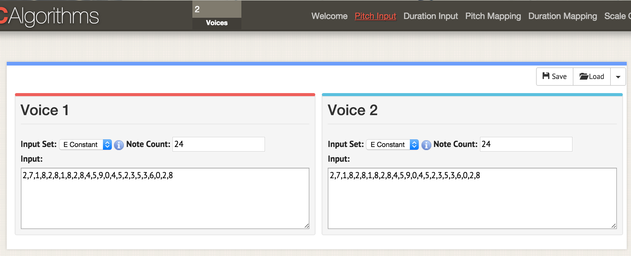
Let's go back to the beginning and load both data columns into this template:
  # Of Voices, Text Area Name, Text Area Data
 2, morphBox,
 , areaPitch1,
 , areaPitch2,
Here we are on the page with the 'pitch input' parameters. At the top of the window, enter two voices, now on any page with parameters two windows open for two voices. As before, we load the data in CSV format, but the file needs to be formatted so that the values of 'areaPitch1' and 'areaPitch2' are indicated there. Data for the first voice will appear on the left, and the second - on the right.
If we have a few voices, what to bring to the fore? Please note that with this approach, our voice acting does not take into account the distance between points in the real world. If taken into account, it will greatly affect the result. Of course, the distance is not necessarily tied to geography - it can be tied to time. The following tool will allow you to clearly indicate this factor when dubbing.
Briefly about configuring Python
This section of the tutorial will require Python. If you have not experimented with this language yet, you will have to spend some time getting to know the command line . See also the module installation quick start guide .
On Macs, Python is already installed. You can check: press COMMAND and space, enter
terminal in the search window and click on the terminal application. The $ type python —version will show which version of Python you have installed. In the article we work with Python 2.7, the code was not checked in Python 3.Windows users need to install Python themselves: start from this page , although everything is a bit more complicated than what is written there. First, you need to download the
.msi file (Python 2.7). Run the installer, it will be installed in a new directory, for example, C:\Python27\ . Then you need to register this directory in the paths, that is, tell Windows where to look for Python when you start the Python program. There are several ways to do this. Perhaps the easiest way to find Powershell on your computer is (enter 'powershell' in the Windows search box). Open Powershell and in the command line, paste it in its entirety: [Environment] :: SetEnvironmentVariable ("Path", "$ env: Path; C: \ Python27 \; C: \ Python27 \ Scripts \", "User") If nothing happens by pressing Enter, then the command worked. To test, open a command prompt (here are 10 ways to do this ) and type
python --version . A response should be displayed indicating Python 2.7.10 or a similar version.The last piece of the puzzle is a program called
Pip . Mac users can install it with a command in the sudo easy_install pip terminal. Windows users will have a little more difficult. First, right-click and save the file by this link (if you simply click on the link, the code get-pip.py opens in the browser). Keep it somewhere handy. Open a command prompt in the directory where you saved get-pip.py . Then type python get-pip.py on the command line.When you have Python code that you want to run, paste it into a text editor and save the file with the extension
.py . This is a text file, but the file extension tells the computer to use to interpret Python. It is launched from the command line, where the name of the interpreter is first specified, and then the file name: python my-cool-script.py .MIDITime
MIDITime is a Python package developed by Reveal News (formerly known as the Center for Investigative Journalism). Repository on Github . MIDITime is designed specifically for processing time series (that is, a sequence of observations collected over time).
While Musicalgorithms has a more or less intuitive interface, here the advantage is open source. More importantly, the previous tool does not know how to take into account data taking into account historical time. MIDITime allows you to cluster information on this factor.
Suppose we have a historical diary to which the thematic model has been applied. The resulting output may contain diary entries in the form of lines, and in the columns will be the percentage contribution of each topic. In this case, listening to the values will help to understand such patterns of thinking from the diary, which can not be transferred as a graph. Emissions or repetitive musical patterns that are not visible on the chart are immediately noticeable.
MIDITime installation
Installation with one pip command:
$ pip install miditime for poppies;
$ sudo pip install miditime under Linux;
> python pip install miditime under Windows (if the instruction does not work, you can try this helper program to install Pip).
Practice
Consider an example script. Open a text editor, copy and paste this code:
#!/usr/bin/python from miditime.miditime import MIDITime # NOTE: this import works at least as of v1.1.3; for older versions or forks of miditime, you may need to use # from miditime.MIDITime import MIDITime # Instantiate the class with a tempo (120bpm is the default) and an output file destination. mymidi = MIDITime(120, 'myfile.mid') # Create a list of notes. Each note is a list: [time, pitch, attack, duration] midinotes = [ [0, 60, 200, 3], #At 0 beats (the start), Middle C with attack 200, for 3 beats [10, 61, 200, 4] #At 10 beats (12 seconds from start), C#5 with attack 200, for 4 beats ] # Add a track with those notes mymidi.add_track(midinotes) # Output the .mid file mymidi.save_midi() Save the script as
music1.py . In a terminal or command line, run it: $ python music1.py A new file
myfile.mid will be created in the myfile.mid . You can open it for listening using Quicktime or Windows Media Player (and add tools to GarageBand or LMMS there ).Music1.py imports miditime (do not forget to install it before running the script: pip install miditime ). Then sets the pace. All notes are listed separately, where the first number is the start time of the playback, the pitch (i.e., the note itself!), How strongly or rhythmically the note (attack) is played and its duration. Then the notes are recorded on the track, and the track itself is recorded in the file myfile.mid .Play with the script, add more notes. Here are the notes for the song 'Baa Baa Black Sheep':
  D, D, A, A, B, B, B, B, A
 Baa, Baa, black, sheep, have, you, any, wool?
Can you write instructions for the computer to play the melody (here's a chart to help)?
By the way . There is a special text file format for describing music called ABC Notation . It is beyond the scope of this article, but a scoring script can be written, say, in spreadsheets, comparing the values of notes in ABC notation (if you have ever used the IF - THEN construct in Excel, you have an idea how this is done) and then through sites like this, the ABC notation is converted to a .mid file.
Upload your own data
This file contains a selection of the thematic model diaries of John Adams for the Macroscope site. Here only the strongest signals were left, rounding up the values in the columns to two decimal places. To insert this data into the Python script, you need to format it in a special way. The hardest thing is the date field.
For this lesson, we leave the variable names and the rest unchanged from the script with an example. The sample is designed to process earthquake data; therefore, here “magnitude” can be represented as our “contribution of the theme”.
  my_data = [
     {'event_date': <datetime object>, 'magnitude': 3.4},
     {'event_date': <datetime object>, 'magnitude': 3.2},
     {'event_date': <datetime object>, 'magnitude': 3.6},
     {'event_date': <datetime object>, 'magnitude': 3.0},
     {'event_date': <datetime object>, 'magnitude': 5.6},
     {'event_date': <datetime object>, 'magnitude': 4.0}
 ]
For formatting data, you can use regular expressions, and even easier - spreadsheets. Copy the element with the theme contribution value to the new sheet and leave the columns left and right. In the example below, I placed it in column D, and then filled the rest:
| A | B | C | D | E | |
|---|---|---|---|---|---|
| one | {'event_date': datetime | (1753,6,8) | , 'magnitude': | 0.0024499630 | }, |
| 2 | |||||
| 3 |
Then copy and paste the immutable elements by filling in the entire column. The element with the date must be in the format (year, month, day). After filling the table, it can be copied and pasted into a text editor, making it part of the
my_data array, for example: my_data = [
{'event_date': datetime (1753,6,8), 'magnitude': 0.0024499630},
{'event_date': datetime (1753,6,9), 'magnitude': 0.0035766320},
{'event_date': datetime (1753,6,10), 'magnitude': 0.0022171550},
{'event_date': datetime (1753,6,11), 'magnitude': 0.0033220150},
{'event_date': datetime (1753,6,12), 'magnitude': 0.0046445900},
{'event_date': datetime (1753,6,13), 'magnitude': 0.0035766320},
{'event_date': datetime (1753,6,14), 'magnitude': 0.0042241550}
] Note that there is no comma at the end of the last line.
The final script will look something like this if you use the example from the Miditime page itself (the code snippets below are interrupted by comments, but they should be pasted together into a text editor as one file):
from miditime.MIDITime import MIDITime from datetime import datetime import random mymidi = MIDITime(108, 'johnadams1.mid', 3, 4, 1) Values after MIDITime are set as
MIDITime(108, 'johnadams1.mid', 3, 4, 1) , here:- beats per minute (108),
- output file ('johnadams1.mid'),
- the number of seconds in the music to represent one year in history (3 seconds per calendar year, so the diary entries for 50 years are scaled to a melody of 50 × 3 seconds, that is, two and a half minutes),
- the basic octave for music (the average C is usually represented as C5, so here 4 corresponds to an octave one lower than the reference),
- and the number of octaves to match the heights.
Now we transfer the data to the script by loading it into the array
my_data : my_data = [ {'event_date': datetime(1753,6,8), 'magnitude':0.0024499630}, {'event_date': datetime(1753,6,9), 'magnitude':0.0035766320}, ... here we insert all the data and do not forget to delete the comma at the end of the last line of
event_date , and after the data put the terminating bracket on a separate line: {'event_date': datetime(1753,6,14), 'magnitude':0.0042241550} ] then insert the timing:
my_data_epoched = [{'days_since_epoch': mymidi.days_since_epoch(d['event_date']), 'magnitude': d['magnitude']} for d in my_data] my_data_timed = [{'beat': mymidi.beat(d['days_since_epoch']), 'magnitude': d['magnitude']} for d in my_data_epoched] start_time = my_data_timed[0]['beat'] This code sets the timing between different diary entries; if the diaries are close to each other in time, the corresponding notes will also be closer. Finally, we determine how the data is compared to the height. The initial values are indicated in percents in the range from 0.01 (i.e. 1%) to 0.99 (99%), so
scale_pct set between 0 and 1. If we have no percentages, then we use the lowest and the highest values. Thus, we insert the following code: def mag_to_pitch_tuned(magnitude): scale_pct = mymidi.linear_scale_pct(0, 1, magnitude) # Pick a range of notes. This allows you to play in a key. c_major = ['C', 'C#', 'D', 'D#', 'E', 'E#', 'F', 'F#', 'G', 'G#', 'A', 'A#', 'B', 'B#'] #Find the note that matches your data point note = mymidi.scale_to_note(scale_pct, c_major) #Translate that note to a MIDI pitch midi_pitch = mymidi.note_to_midi_pitch(note) return midi_pitch note_list = [] for d in my_data_timed: note_list.append([ d['beat'] - start_time, mag_to_pitch_tuned(d['magnitude']), random.randint(0,200), # attack random.randint(1,4) # duration, in beats ]) and the last fragment to save the data to a file:
# Add a track with those notes mymidi.add_track(midinotes) # Output the .mid file mymidi.save_midi() Save this file with a new name and the extension
.py .For each column in the source data we make a unique script and do not forget to change the name of the output file ! You can then upload individual midi files to GarageBand or LMMS for instrumentation. Here is the complete diary of John Adams .
Sonic pi
Processing unique midi in GarageBand or another music editor means moving from simple voice over to the art of music. This final section of the article is not a complete guide to using the Sonic Pi , but rather an introduction to an environment that allows you to encode and play back data in the form of music in real time (see video for an example of coding with real-time playback ). The tutorials built into the program will show how to use the computer as a musical instrument (you enter Ruby code into the built-in editor, and the interpreter loses the result immediately).
Why do you need it? As you can see from this tutorial, as data is played out, you begin to make decisions about how to translate data into sound. These decisions reflect implicit or explicit decisions about which data is relevant. There is a continuum of “objectivity,” if you will. On the one hand, the historical data that has been voiced, on the other hand, the view of the past is as exciting and personal as any well-done public lecture. Voicing allows you to actually hear the data stored in the documents: it is a kind of public story. The musical performance of our data ... just imagine!
Here I offer a code snippet for importing data, which is simply a list of values saved as csv. Thanks to the librarian of George Washington University Laura Vrubel, who posted her experiments on dubbing library operations on gist.github.com .
In this sample (thematic model generated from the Jesuit Relation ) there are two themes. The first line contains the headings 'topic1' and 'topic2'.
Practice
Follow the built-in guides of the Sonic Pi until you get familiar with the interface and features (all of these tutorials are collected here ; you can also listen to an interview with Sam Aaron, the creator of Sonic Pi). Then in the new buffer (editor window) copy the following code (again, separate fragments should be collected in one script):
require 'csv' data = CSV.parse(File.read("/path/to/your/directory/data.csv"), {:headers => true, :header_converters => :symbol}) use_bpm 100 Remember that
path/to/your/directory/ is the actual location of your data on the computer. Make sure the file is really called data.csv , or edit this line in the code.Now let's load this data into the musical composition:
#this bit of code will run only once, unless you comment out the line with #'live_loop', and also comment out the final 'end' at the bottom # of this code block #'commenting out' means removing the # sign. # live_loop :jesuit do data.each do |line| topic1 = line[:topic1].to_f topic2 = line[:topic2].to_f use_synth :piano play topic1*100, attack: rand(0.5), decay: rand(1), amp: rand(0.25) use_synth :piano play topic2*100, attack: rand(0.5), decay: rand(1), amp: rand(0.25) sleep (0.5) end The first few rows load data columns; then we indicate which sample of sound we want to use (piano), and then indicate to play the first theme (topic1) according to the specified criteria: for the strength of the note playing (attack) a random value less than 0.5 is selected; for decay (decay) - random value less than 1; for amplitude, a random value of less than 0.25.
See the line with multiplication by one hundred (
*100 )? It takes our data value (decimal) and turns it into an integer. In this passage, the number is directly equivalent to a note. If the lowest note is 88, and the highest is 1, then this approach is a bit problematic: we actually do not display any pitch here! In this case, you can use Musicalgorithms to display the height, and then transfer these values back to Sonic Pi. In addition, since this code is more or less standard Ruby, you can apply the usual methods of data normalization, and then make a linear comparison of your values with a range of 1–88. For a start, take a good look at Steve Lloyd's work on dubbing weather data with Sonic Pi.And the last thing to note here: the value of 'rand' (random) allows you to add a bit of “humanity” to the music in terms of dynamics. Do the same for topic2.
You can also specify the rhythm (beats per minute), loops, samples, and other effects that Sonic Pi supports. The location of the code affects the playback: for example, if placed before the above data block, it will play first. For example, if you
use_bpm 100insert the following after the line : #intro bit sleep 2 sample :ambi_choir, attack: 2, sustain: 4, rate: 0.25, release: 1 sleep 6 ... then get a little musical introduction. The program waits 2 seconds, plays the sample 'ambi_choir', then waits another 6 seconds before playing our data. If you want to add a little sinister drum throughout the melody, put the following bit (before your own data):
#bit that keeps going throughout the music live_loop :boom do with_fx :reverb, room: 0.5 do sample :bd_boom, rate: 1, amp: 1 end sleep 2 end The code is pretty clear: a looped sample of 'bd_boom' with a reverberation sound effect at a certain speed. Pause between cycles of 2 seconds.
As for “real-time coding,” this means that you can make changes to the code while simultaneously playing back those changes . Do not like what you hear? Immediately change the code!
The study of Sonic Pi can be started from this seminar . See also the report of Laura Vrubel on attending the seminar, which also describes her work in this area and the work of her colleagues.
Nothing new under the sun
And I repeat again: it is not necessary to think that we, with our algorithmic approach, are at the forefront of science. In 1978, a scientific article was published on the 18th century “musical dice”, where bone rolls determined the recombination of previously written pieces of music. Robin Newman studied and coded some of these games for Sonic Pi . For Newman musical notation uses a tool that can be described as Markdown + Pandoc, and for conversion into notes - Lilypond . So all the themes on our blog The Programming Historian have a long history!
Conclusion
When dubbing, we see that our data often reflects not so much history as its interpretation in our performance. This is partly due to the novelty and artistic nature necessary to translate data into sound. But it also strongly distinguishes sound interpretation from traditional visualization. Maybe the generated sounds will never rise to the level of "music"; but if they help change our understanding of the past and influence others, then the effort is worth it. As Trevor Owens would say, “Sounding is a discovery of a new, not a justification of the known .”
Terms
- MIDI : . , ( ). . MIDI- , .
- MP3 : , .
- : ( C . .)
- :
- : ( , , . .)
- :
- Amplitude : roughly speaking, the volume of the note
Source: https://habr.com/ru/post/454318/
All Articles