First model: Fashion MNIST dataset
Full course in Russian can be found at this link .
The original English course is available here .

The release of new lectures is scheduled every 2-3 days.
- So, we are again with you and with us is still Sebastian. We just want to discuss fully connected layers, those same Dense layers. Before that, I would like to ask one question. What are the boundaries and what are the main obstacles that will stand in the way of the development of deep learning and will have the greatest impact on it in the next 10 years? Everything changes so fast! What do you think will be the very next “big thing” (big thing - breakthrough)?
- I would call two things. The first is general artificial intelligence (general AI) for performing more than one task. This is great! People can do more than one task and never have to do the same thing. The second is the introduction of technology to the market. For me, a feature of machine learning is that it provides computers with the opportunity to observe and find patterns in the data, helping people become the best in the field - at the expert level! Machine learning can be used in jurisprudence, medicine, autonomous cars. Develop such applications, because they can bring a huge amount of money, but what is most important in this all - you have the opportunity to make the world much better.
- I really like the way everything you said is formed into a single picture of the deep learning and its application - this is just a tool that can help you solve a specific task.
- Yes it is! Incredible tool, right?
- Yes, yes, I completely agree with you!
- Almost like a human brain!
- You mentioned medical applications in our first interview, in the first part of the video course. In which applications, in your opinion, the use of deep learning is the most delightful and surprising?
- Lots of! Highly! Medicine is in the short list of areas that are actively using deep learning. I lost my sister a few months ago, she was sick with cancer, which is very sad. I think there are many diseases that could be detected earlier - in the early stages, giving them the opportunity to cure or slow down their development. The idea, in essence, is to transfer some tools to the house (smart home) so that it is possible to detect such deviations in health long before the moment when the person himself sees them. I would also add - everything is repetitive, any office work where you perform the same type of actions over and over again, for example, bookkeeping. Even I, as the CEO, do a lot of repetitive actions. It would be great to automate them, even work with postal correspondence!
- I can not disagree with you! In this lesson we will introduce students to the course with a layer of a neural network called a dense-layer. Could you tell us more about what you think about full connected layers?
- So, let's start with the fact that each network can be connected in different ways. Some of them may have very dense connectivity, which allows you to get some benefit when scaling and "win" from large networks. Sometimes you don't know how many links you need, so you connect everything with everything — this is called a fully connected layer. I add that this approach has much more power and potential than something more structured.
- Totally agree with you! Thanks for helping us learn a little more about full connected layers. I look forward to the moment when we finally get down to their implementation and writing code.
- Enjoy! It will be really fun!
- Welcome back! In the last lesson, you figured out how to build your first neural network using TensorFlow and Keras, how neural networks work and how the workout (training) process is organized. In particular, we saw how to train a model to convert degrees Celsius to degrees Fahrenheit.

')
- We also got acquainted with the concept of fully connected layers (dense-layers), the most important layer in neural networks. But in this lesson we will do much cooler things! In this lesson we will develop a neural network that can recognize elements of clothing and images. As we mentioned earlier, machine learning uses input data called “attributes” (features, properties) and output data called “labels” (labels) by which the model learns and finds the transformation algorithm. Therefore, first, we need many examples to train the neural network to recognize the various elements of clothing. Let me remind you that the example for learning is a pair of values - the input feature and output label, which are fed to the input of the neural network. In our new example, the image will be the input data, and the output label should be the category of clothing to which the item of clothing shown in the picture belongs. Fortunately, such a data set already exists. It is called Fashion MNIST. We will take a closer look at this dataset in the next section.
Welcome to the world of the MNIST dataset! So, our set consists of 28x28 images, each pixel of which is a shade of gray.
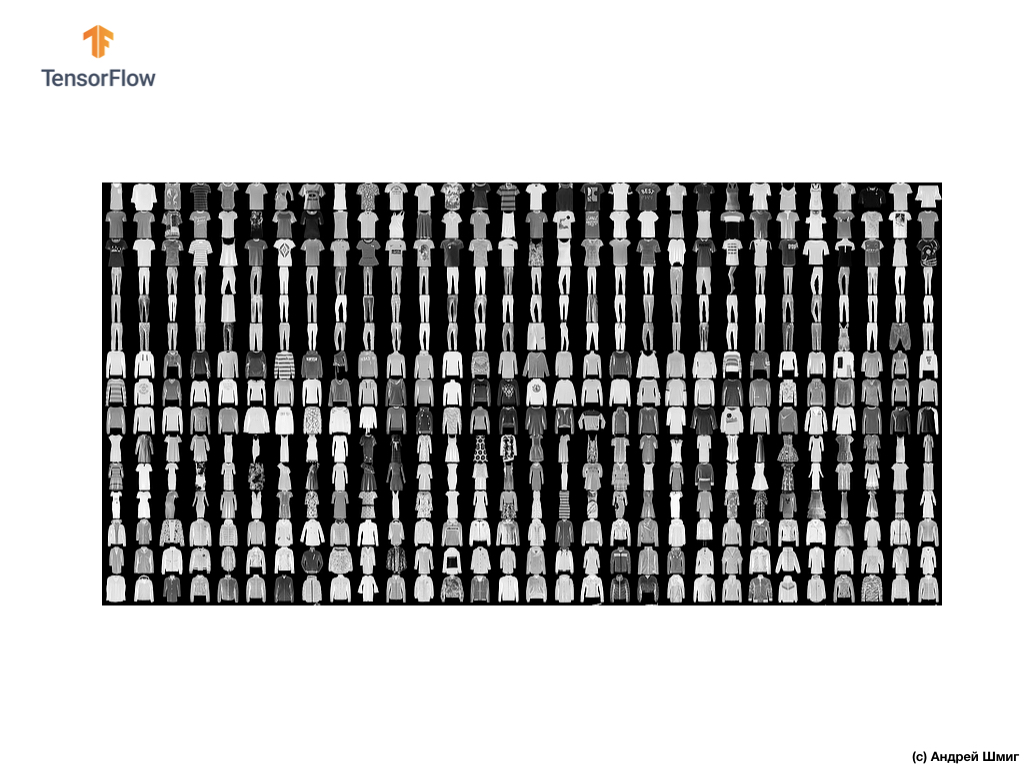
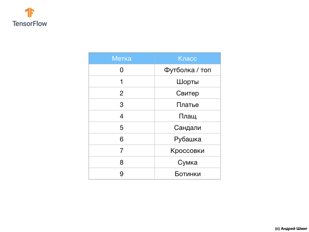
The data set contains images of T-shirts, tops, sandals, and even shoes. Here is a complete list of what our MNIST dataset contains:
Each input image corresponds to one of the above tags. The MNIST Fashion dataset contains 70,000 images, so we have a place to start and work with. Of these 70,000, we will use 60,000 to train the neural network.
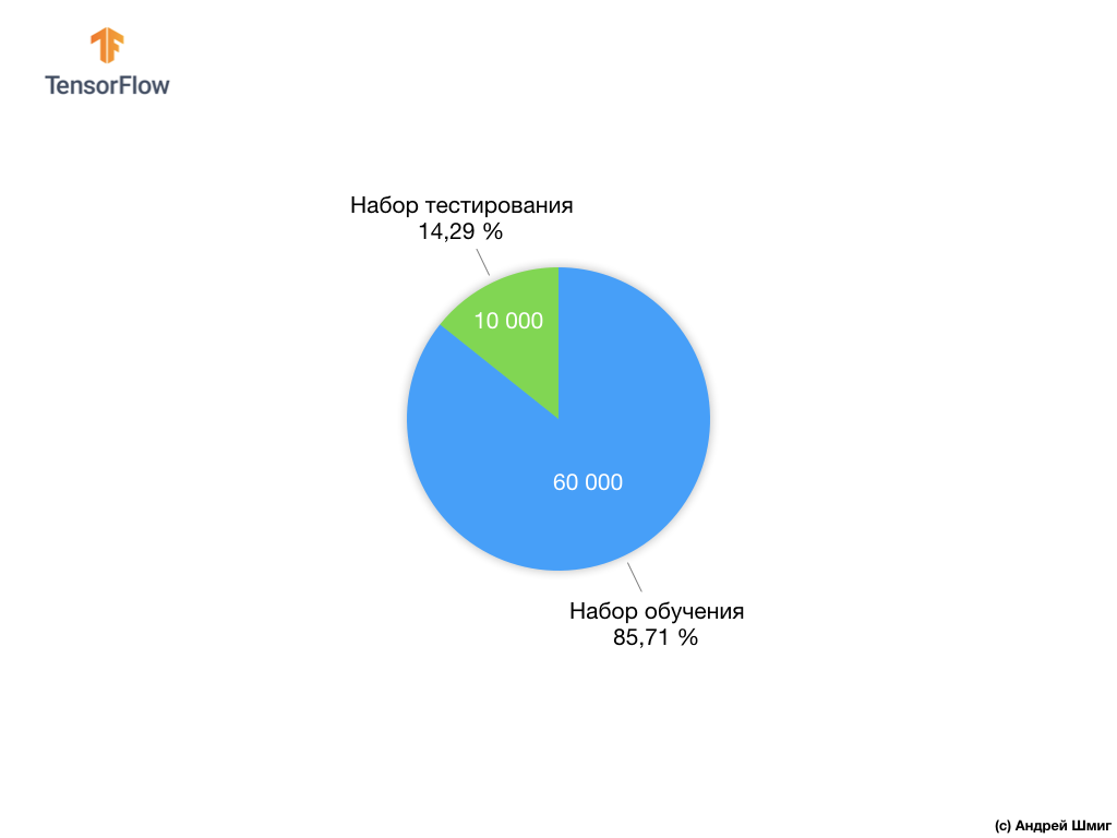
And we will use the remaining 10,000 elements in order to check how well our neural network has learned to recognize the elements of clothing. A little later, we will explain why we divided the data set into a training set and into a testing set.
So, here is our Fashion MNIST dataset.
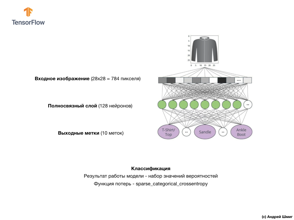
Remember, each image in the dataset is a 28x28 image in grayscale, which means that each image is 784 bytes in size. Our task is to create a neural network that receives these 784 bytes at the input, and returns to which category of clothing out of 10 that the input element belongs to.
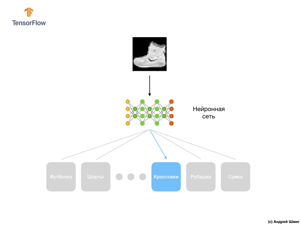
In this lesson, we will use a deep neural network that will learn to classify images from the Fashion MNIST dataset.
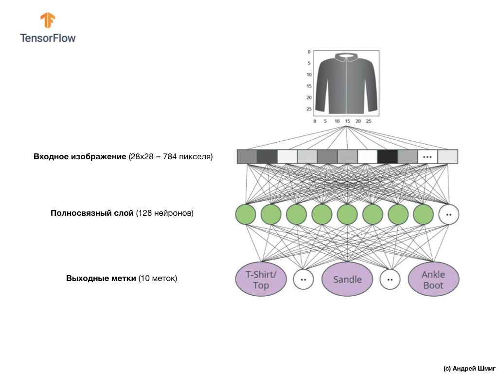
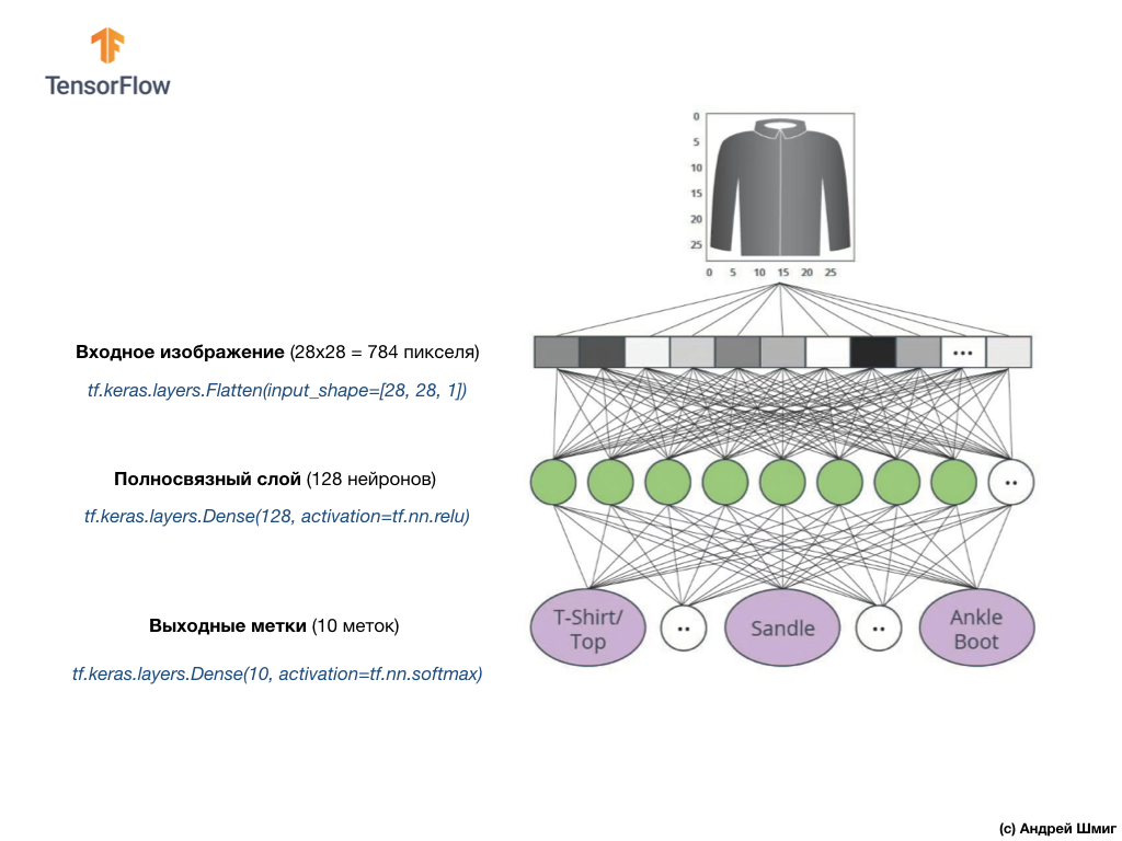
The image above shows what our neural network will look like. Let's take a closer look at it.
The input value of our neural network is a one-dimensional array with a length of 784, an array of exactly that length, for the reason that each image is 28x28 pixels (= 784 pixels in the image), which we transform into a one-dimensional array. The process of converting a 2D image into a vector is called flattening and is implemented by means of a smoothing layer — a flatten layer.
Smoothing can be done by creating the appropriate layer:
This layer converts a 2D image of 28x28 pixels (for each pixel there is 1 byte for shades of gray) into a 1D array consisting of 784 pixels.
Input values will be fully connected with our first
Here is how the creation of this layer in the code will look like:
Stop! What is this
Finally, our last layer, also known as the output layer, consists of 10 neurons. It consists of 10 neurons because our Fashion MNIST dataset contains 10 categories of clothing. Each of these 10 output values will represent the probability that the image fed to the input belongs to this category of clothing. In other words, these values reflect the “confidence” of the model in the correctness of the prediction and the correlation of the submitted image with a certain of 10 categories of clothing at the output. For example, what is the probability that the image of a dress, sneakers, shoes, etc.
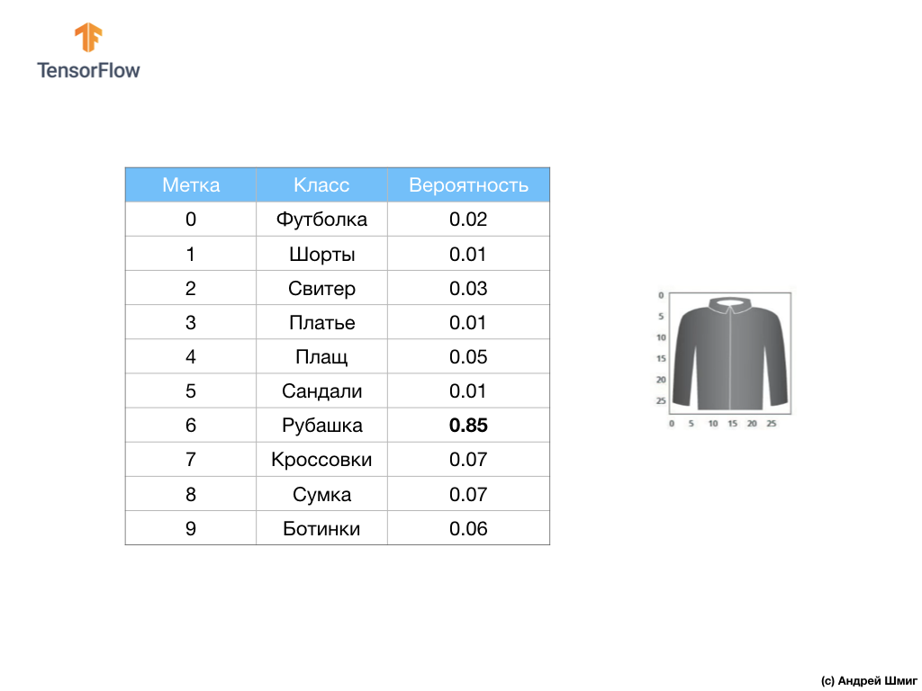
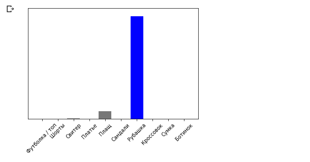
For example, if an image of a shirt is submitted to the input of our neural network, the model can give us results like the ones you see in the image above - the probability of matching the input image with the output label.
If you pay attention, you will notice that the greatest probability - 0.85 refers to the mark 6, which corresponds to the shirt. The model is 85% sure that the image on the shirt. Usually those things that will look like shirts will also have a high estimate of probability, and the least similar things will have the lowest estimate of probability.
Since all 10 output values correspond to probabilities, when summing all these values we get 1. These 10 values are also called probability distributions.
Now we need an output layer to calculate the same probabilities for each label.
And we will do this with the following command:
In fact, whenever we create neural networks that solve classification problems, we always use a fully connected layer as the last layer of the neural network. The last layer of the neural network must contain the number of neurons equal to the number of classes, belonging to which we define and use the softmax activation function.
In this lesson we talked about
The
The conversion of degrees Celsius to degrees Fahrenheit is a linear problem, because the expression
Let's go over the new terms introduced in this lesson:
When training a model any model in machine learning it is always necessary to divide the data set into at least two different sets - the data set used for training and the data set used for testing. In this part, we will understand why it is worth doing so.
Let's recall how we distributed our data set from Fashion MNIST consisting of 70,000 copies.
We suggested dividing 70,000 into two parts - leaving 60,000 for training in the first part and 10,000 for testing in the second part. The need for such an approach is caused by the following fact: after the model has been trained in 60,000 copies, it is necessary to check the results and the effectiveness of its work on such examples that were not yet in the data set on which the model was trained.
In a way, it is like passing an exam at school. Before you take the exam, you are diligently engaged in solving problems of a particular class. Then, in the exam, you encounter the same class of problems, but other input data. There is no point in giving the same data to the input that was used during the training session, otherwise the task will be to memorize solutions, and not to find a solution model. That is why in the exams you are confronted with such tasks that were not previously in the training program. Only in this way can you check whether the model has learned the general solution or not.
The same thing happens with machine learning. You show some data that represents a certain class of problems that you want to learn to solve. In our case, with the data set from Fashion MNIST, we want the neural network to be able to determine the category to which the item of clothing in the image belongs. That is why we are training our model with 60,000 examples that contain all categories of clothing items. After a workout, we want to test the model’s effectiveness, so we feed the remaining 10,000 items of clothing that the model hasn’t yet seen. If we decided not to do this, do not test on 10,000 examples, we would not be able to say with confidence whether our model had actually learned to determine the class of an item of clothing or she remembered all pairs of input + output values.
That is why in machine learning we always have a data set for training and a data set for testing.
The TensorFlow Kit Kit provides a collection of ready-to-use training data.
Data sets are usually divided into several blocks, each of which is used at a certain stage of training and testing the effectiveness of the neural network. In this part we are talking about:
Consider another set of data, which I call the validation dataset. This data set is not used to train a model, only during a workout. So, after our model has gone through several training cycles, we feed our test data set to it and look at the results. For example, if during a workout the value of the loss function decreases, and the accuracy deteriorates on the test data set, then this means that our model simply remembers the pairs of input-output values.
The test data set is reused at the very end of the workout to measure the final accuracy of the model predictions.
More information about the training and test data sets can be found in Google Crash Course .
Link to the original CoLab in English and link to Russian CoLab .
In this part of the lesson, we will build and train the neural network to classify images of items of clothing, such as dresses, sneakers, shirts, t-shirts, etc.
All right, if some moments will be incomprehensible. The purpose of this course is to introduce you to TensorFlow and in parallel to explain the algorithms of its work and develop a common understanding of projects using TensorFlow, and not go into the details of implementation.
In this part, we use
We need a TensorFlow dataset , an API that simplifies loading and accessing datasets provided by several services. We will also need several auxiliary libraries.
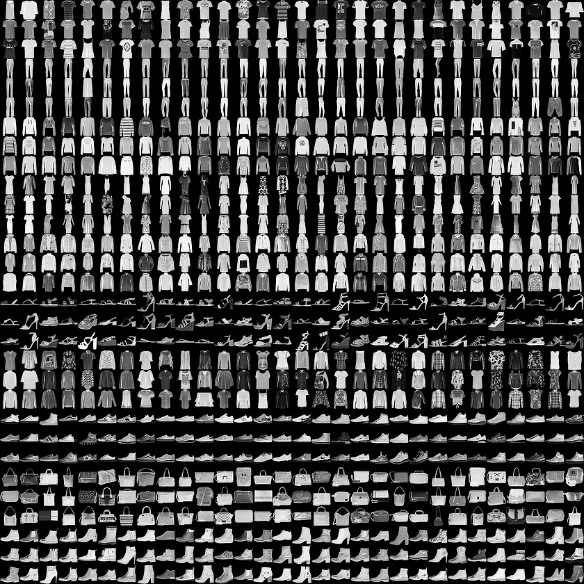
This example uses the MNIST Fashion dataset, which contains 70,000 images of clothing items in 10 categories in grayscale. The images contain clothes in low resolution (28x28 pixels), as shown below:
Fashion MNIST is used as a replacement for the classic MNIST data set — most often used as “Hello, World!” In machine learning and computer vision. The MNIST dataset contains handwritten numbers (0, 1, 2, etc.) in the same format as the clothing elements in our example.
In our example, we use Fashion MNIST because of the diversity and because this task is more interesting from the point of view of implementation than the solution of a typical problem on the MNIST data set. Both data sets are small enough, therefore, they are used to verify the correct operation of the algorithm. Excellent data sets for starting learning machine learning, testing and debugging code.
We will use 60,000 images to train the network and 10,000 images to test the accuracy of training and image classification. You can directly access the MNIST Fashion dataset via TensorFlow using the API:
By loading a data set we get metadata, a training data set and a test data set.
The images are two-dimensional arrays
Each image belongs to one tag. Since the class names are not contained in the original data set, let's save them for later use when we draw the images:
Let's examine the format and structure of the data presented in the training set before training the model. The following code shows that 60,000 images are in the training dataset, and 10,000 images are in the test set:
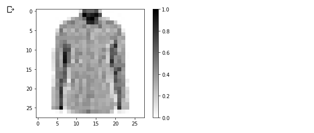
The value of each pixel in the image is in the interval
Let's draw an image to take a look at it:
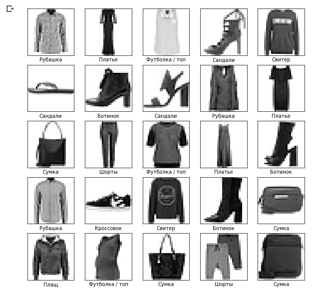
We will display the first 25 images from the training data set and under each image we will indicate to which class it belongs.
Make sure that the data is in the correct format and we are ready to start creating and training the network.
Building a neural network requires adjusting layers, and then building a model with optimization and loss functions.
The basic element in the construction of a neural network is a layer. The layer extracts the view from the data it received at the input. The result of the work of several related layers, we get an idea that makes sense to solve the problem.
Most of the time in deep learning, you will be creating links between simple layers. Most layers, for example, such as tf.keras.layers.Dense have a set of parameters that can be “tailored” during the learning process.
The network consists of three layers:
Before we begin to train the model, it is worth making a few adjustments. These settings are made during model building when calling the compile method:
First, we determine the sequence of actions during training at the training data set:
Training takes place by calling the
(you can ignore the
And here is the conclusion:
In the process of training the model, the value of the loss function and the accuracy metric are displayed for each training iteration. This model achieves an accuracy of around 0.88 (88%) on training data.
Check what accuracy gives the model on the test data. We will use all the examples that we have in the test dataset to verify accuracy.
Conclusion:
As you can see, the accuracy on the test dataset turned out to be less accurate on the training dataset. This is quite normal, since the model was trained on train_dataset data. When the model detects images that it has never seen before (from the train_dataset dataset), it is quite obvious that the classification efficiency will decrease.
We can use the trained model to get predictions for some images.
Conclusion:
In the example above, the model predicted the labels for each test input image. Let's look at the first prediction:
Conclusion:
Recall that model predictions are an array of 10 values. These values describe the “confidence” of the model that the input image belongs to a certain class (clothing item). We can see the maximum value as follows:
Conclusion:
This means that the model showed the greatest confidence that this image belongs to the class with label 6 (class_names [6]). We can check and make sure that the result is true and correct:
We can display all input images and corresponding model predictions in 10 classes:
Let's take a look at the 0th image, the result of the model prediction and the array of predictions.
Let's now display some images with their respective predictions. Correct predictions are blue, incorrect ones are red. The value under the image reflects the percentage of confidence in the model that the input image corresponds to this class. Please note that the result may be incorrect even if the value of “confidence” is large.
Use the trained model to predict the label for a single image:
Conclusion:
Models in
Conclusion:
Now let's predict the result:
Conclusion:
The model.predict method returns a list of lists (array of arrays), each for an image from a block of input data. We get the only result for our single input image:
Conclusion:
As previously, the model predicted label 6 (shirt).
Experiment with different models and see how the accuracy will change. In particular, try changing the following parameters:
Do not forget to activate the GPU so that all the calculations are faster (
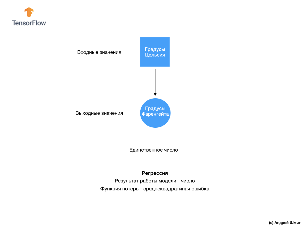
- At this stage, we have already encountered two types of neural networks. Our first neural network has learned to convert degrees Celsius to degrees Frenheit, returning a single value that can be in a wide range of numerical values.
Our second neural network returns 10 probability values that represent the network’s confidence that the image fed to the input corresponds to a certain class.
Neural networks can be used to solve various kinds of problems.
The first class of problems that we solved with the prediction of a single value is called regression.. The conversion of degrees Celsius to degrees Fahrenheit is one example of the task of this class. Another example of this class of tasks may be the problem of determining the value of a house by room number, total area, location, and other characteristics.
The second class of problems, which we considered in this lesson by classifying images into existing categories, is called classification . According to the input data, the model will return the probability distribution (the “confidence” of the model that the input value belongs to this class). In this lesson, we developed a neural network that classified items of clothing into 10 categories, and in the next lesson we will learn to determine who the dog or cat is depicted in the photo, this task also applies to the classification task.
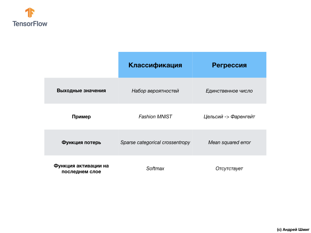
Let's summarize and note the difference between these two classes of problems - regression and classification .
Congratulations, you learned two types of neural networks! Get ready for the next lecture, where we will study a new type of neural networks - convolutional neural networks (CNN, convolutional neural networks).
In this lesson, we taught the neural network to classify images with items of clothing. To do this, we used the MNIST Fashion dataset, which contains 70,000 images of clothing items. 60,000 of which we used to train the neural network, and the remaining 10,000 to test its performance. In order to feed these images to the input of our neural network, we needed to convert them (smooth out) from a 28x28 2D format to a 1D format of 784 elements. Our network consisted of a fully connected layer of 128 neurons and an output layer of 10 neurons, corresponding to the number of tags (classes, categories of elements of clothing). These 10 output values represented the probability distribution for each class. Softmax activation functioncounted the probability distribution.
We also learned about the differences between regression and classification .
... and standard call-to-action - subscribe, put a plus and share :)
YouTube
Telegram
In contact with
The original English course is available here .
The release of new lectures is scheduled every 2-3 days.
Interview with Sebastian Trun, CEO Udacity
- So, we are again with you and with us is still Sebastian. We just want to discuss fully connected layers, those same Dense layers. Before that, I would like to ask one question. What are the boundaries and what are the main obstacles that will stand in the way of the development of deep learning and will have the greatest impact on it in the next 10 years? Everything changes so fast! What do you think will be the very next “big thing” (big thing - breakthrough)?
- I would call two things. The first is general artificial intelligence (general AI) for performing more than one task. This is great! People can do more than one task and never have to do the same thing. The second is the introduction of technology to the market. For me, a feature of machine learning is that it provides computers with the opportunity to observe and find patterns in the data, helping people become the best in the field - at the expert level! Machine learning can be used in jurisprudence, medicine, autonomous cars. Develop such applications, because they can bring a huge amount of money, but what is most important in this all - you have the opportunity to make the world much better.
- I really like the way everything you said is formed into a single picture of the deep learning and its application - this is just a tool that can help you solve a specific task.
- Yes it is! Incredible tool, right?
- Yes, yes, I completely agree with you!
- Almost like a human brain!
- You mentioned medical applications in our first interview, in the first part of the video course. In which applications, in your opinion, the use of deep learning is the most delightful and surprising?
- Lots of! Highly! Medicine is in the short list of areas that are actively using deep learning. I lost my sister a few months ago, she was sick with cancer, which is very sad. I think there are many diseases that could be detected earlier - in the early stages, giving them the opportunity to cure or slow down their development. The idea, in essence, is to transfer some tools to the house (smart home) so that it is possible to detect such deviations in health long before the moment when the person himself sees them. I would also add - everything is repetitive, any office work where you perform the same type of actions over and over again, for example, bookkeeping. Even I, as the CEO, do a lot of repetitive actions. It would be great to automate them, even work with postal correspondence!
- I can not disagree with you! In this lesson we will introduce students to the course with a layer of a neural network called a dense-layer. Could you tell us more about what you think about full connected layers?
- So, let's start with the fact that each network can be connected in different ways. Some of them may have very dense connectivity, which allows you to get some benefit when scaling and "win" from large networks. Sometimes you don't know how many links you need, so you connect everything with everything — this is called a fully connected layer. I add that this approach has much more power and potential than something more structured.
- Totally agree with you! Thanks for helping us learn a little more about full connected layers. I look forward to the moment when we finally get down to their implementation and writing code.
- Enjoy! It will be really fun!
Introduction
- Welcome back! In the last lesson, you figured out how to build your first neural network using TensorFlow and Keras, how neural networks work and how the workout (training) process is organized. In particular, we saw how to train a model to convert degrees Celsius to degrees Fahrenheit.
')
- We also got acquainted with the concept of fully connected layers (dense-layers), the most important layer in neural networks. But in this lesson we will do much cooler things! In this lesson we will develop a neural network that can recognize elements of clothing and images. As we mentioned earlier, machine learning uses input data called “attributes” (features, properties) and output data called “labels” (labels) by which the model learns and finds the transformation algorithm. Therefore, first, we need many examples to train the neural network to recognize the various elements of clothing. Let me remind you that the example for learning is a pair of values - the input feature and output label, which are fed to the input of the neural network. In our new example, the image will be the input data, and the output label should be the category of clothing to which the item of clothing shown in the picture belongs. Fortunately, such a data set already exists. It is called Fashion MNIST. We will take a closer look at this dataset in the next section.
Fashion MNIST dataset
Welcome to the world of the MNIST dataset! So, our set consists of 28x28 images, each pixel of which is a shade of gray.
The data set contains images of T-shirts, tops, sandals, and even shoes. Here is a complete list of what our MNIST dataset contains:
Each input image corresponds to one of the above tags. The MNIST Fashion dataset contains 70,000 images, so we have a place to start and work with. Of these 70,000, we will use 60,000 to train the neural network.
And we will use the remaining 10,000 elements in order to check how well our neural network has learned to recognize the elements of clothing. A little later, we will explain why we divided the data set into a training set and into a testing set.
So, here is our Fashion MNIST dataset.
Remember, each image in the dataset is a 28x28 image in grayscale, which means that each image is 784 bytes in size. Our task is to create a neural network that receives these 784 bytes at the input, and returns to which category of clothing out of 10 that the input element belongs to.
Neural network
In this lesson, we will use a deep neural network that will learn to classify images from the Fashion MNIST dataset.
The image above shows what our neural network will look like. Let's take a closer look at it.
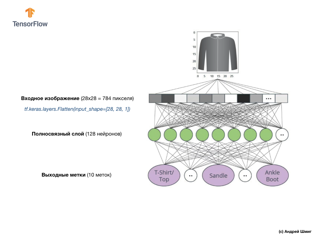
The input value of our neural network is a one-dimensional array with a length of 784, an array of exactly that length, for the reason that each image is 28x28 pixels (= 784 pixels in the image), which we transform into a one-dimensional array. The process of converting a 2D image into a vector is called flattening and is implemented by means of a smoothing layer — a flatten layer.
Smoothing can be done by creating the appropriate layer:
tf.keras.layers.Flatten(input_shape=[28, 28, 1]) This layer converts a 2D image of 28x28 pixels (for each pixel there is 1 byte for shades of gray) into a 1D array consisting of 784 pixels.
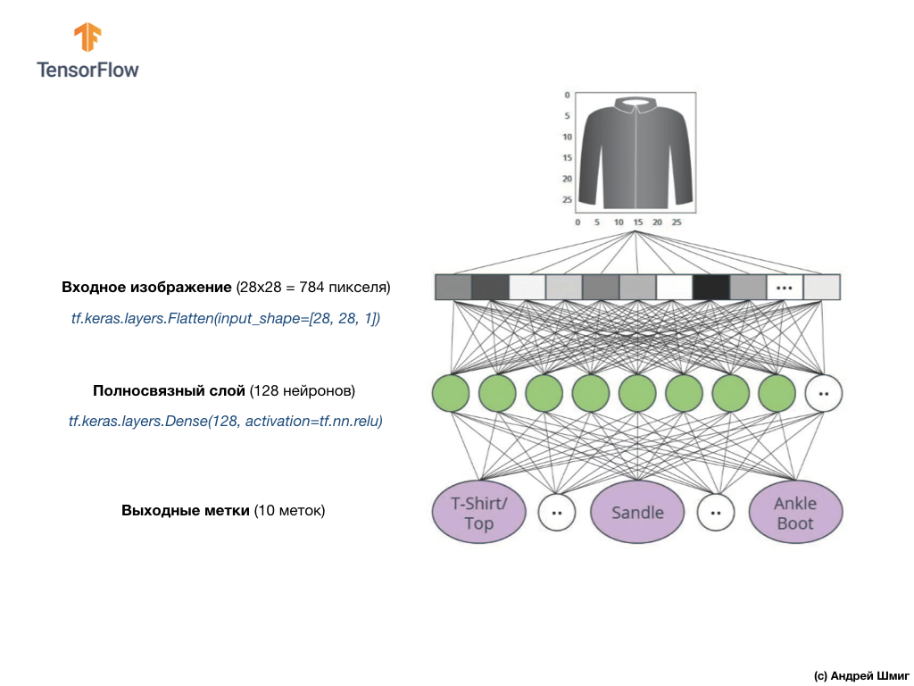
Input values will be fully connected with our first
dense network layer, the size of which we have chosen to be equal to 128 neurons.Here is how the creation of this layer in the code will look like:
tf.keras.layers.Dense(128, activation=tf.nn.relu) Stop! What is this
tf.nn.relu ? We did not use this in our previous example with a neural network when converting degrees Celsius to degrees Fahrenheit! The bottom line is that the current task is much more complicated than the one that was used as an introductory example - converting degrees Celsius to degrees Fahrenheit.ReLU is a mathematical function that we add to our fully connected layer and that gives more power to our network. In fact, this is a small extension for our fully connected layer, which allows our neural network to solve more complex problems. We will not go into details, but you will find more detailed information below.Finally, our last layer, also known as the output layer, consists of 10 neurons. It consists of 10 neurons because our Fashion MNIST dataset contains 10 categories of clothing. Each of these 10 output values will represent the probability that the image fed to the input belongs to this category of clothing. In other words, these values reflect the “confidence” of the model in the correctness of the prediction and the correlation of the submitted image with a certain of 10 categories of clothing at the output. For example, what is the probability that the image of a dress, sneakers, shoes, etc.
For example, if an image of a shirt is submitted to the input of our neural network, the model can give us results like the ones you see in the image above - the probability of matching the input image with the output label.
If you pay attention, you will notice that the greatest probability - 0.85 refers to the mark 6, which corresponds to the shirt. The model is 85% sure that the image on the shirt. Usually those things that will look like shirts will also have a high estimate of probability, and the least similar things will have the lowest estimate of probability.
Since all 10 output values correspond to probabilities, when summing all these values we get 1. These 10 values are also called probability distributions.
Now we need an output layer to calculate the same probabilities for each label.
And we will do this with the following command:
tf.keras.layers.Dense(10, activation=tf.nn.softmax) In fact, whenever we create neural networks that solve classification problems, we always use a fully connected layer as the last layer of the neural network. The last layer of the neural network must contain the number of neurons equal to the number of classes, belonging to which we define and use the softmax activation function.
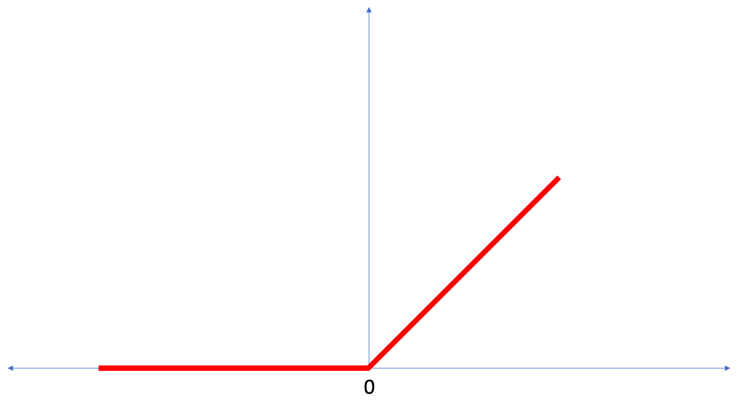
ReLU - neuron activation function
In this lesson we talked about
ReLU as something that expands the capabilities of our neural network and gives it extra power.ReLU is a mathematical function that looks like this:The
ReLU function returns 0 if the input value was a negative value or zero, in all other cases the function will return the original input value.ReLU makes it possible to solve non-linear problems.The conversion of degrees Celsius to degrees Fahrenheit is a linear problem, because the expression
f = 1.8*c + 32 is an equation of a straight line - y = m*x + b . But most of the tasks that we want to solve are non-linear. In such cases, adding the activation function of the ReLU to our fully connected layer can help to cope with such tasks.ReLU is just one type of activation function. There are activation functions such as sigmoid, ReLU, ELU, tanh, but it is ReLU that ReLU most often used as the default activation function. To build and use models that include a ReLU, you do not need to understand how it works inside. If you still want to understand better, we recommend this article .Let's go over the new terms introduced in this lesson:
- Smoothing - the process of converting a 2D image to a 1D vector;
- ReLU is an activation function that allows the model to solve non-linear problems;
- Softmax is a function that calculates probabilities for each possible output class;
- Classification is a class of machine learning tasks used to distinguish between two or more categories (classes).
Training and Testing
When training a model any model in machine learning it is always necessary to divide the data set into at least two different sets - the data set used for training and the data set used for testing. In this part, we will understand why it is worth doing so.
Let's recall how we distributed our data set from Fashion MNIST consisting of 70,000 copies.
We suggested dividing 70,000 into two parts - leaving 60,000 for training in the first part and 10,000 for testing in the second part. The need for such an approach is caused by the following fact: after the model has been trained in 60,000 copies, it is necessary to check the results and the effectiveness of its work on such examples that were not yet in the data set on which the model was trained.
In a way, it is like passing an exam at school. Before you take the exam, you are diligently engaged in solving problems of a particular class. Then, in the exam, you encounter the same class of problems, but other input data. There is no point in giving the same data to the input that was used during the training session, otherwise the task will be to memorize solutions, and not to find a solution model. That is why in the exams you are confronted with such tasks that were not previously in the training program. Only in this way can you check whether the model has learned the general solution or not.
The same thing happens with machine learning. You show some data that represents a certain class of problems that you want to learn to solve. In our case, with the data set from Fashion MNIST, we want the neural network to be able to determine the category to which the item of clothing in the image belongs. That is why we are training our model with 60,000 examples that contain all categories of clothing items. After a workout, we want to test the model’s effectiveness, so we feed the remaining 10,000 items of clothing that the model hasn’t yet seen. If we decided not to do this, do not test on 10,000 examples, we would not be able to say with confidence whether our model had actually learned to determine the class of an item of clothing or she remembered all pairs of input + output values.
That is why in machine learning we always have a data set for training and a data set for testing.
The TensorFlow Kit Kit provides a collection of ready-to-use training data.
Data sets are usually divided into several blocks, each of which is used at a certain stage of training and testing the effectiveness of the neural network. In this part we are talking about:
- training dataset : a dataset designed to train a neural network;
- test dataset : a dataset designed to test the performance of a neural network;
Consider another set of data, which I call the validation dataset. This data set is not used to train a model, only during a workout. So, after our model has gone through several training cycles, we feed our test data set to it and look at the results. For example, if during a workout the value of the loss function decreases, and the accuracy deteriorates on the test data set, then this means that our model simply remembers the pairs of input-output values.
The test data set is reused at the very end of the workout to measure the final accuracy of the model predictions.
More information about the training and test data sets can be found in Google Crash Course .
Practical part in CoLab
Link to the original CoLab in English and link to Russian CoLab .
Classification of images of clothing items
In this part of the lesson, we will build and train the neural network to classify images of items of clothing, such as dresses, sneakers, shirts, t-shirts, etc.
All right, if some moments will be incomprehensible. The purpose of this course is to introduce you to TensorFlow and in parallel to explain the algorithms of its work and develop a common understanding of projects using TensorFlow, and not go into the details of implementation.
In this part, we use
tf.keras - a high-level API for building and training models in TensorFlow.Installing and importing dependencies
We need a TensorFlow dataset , an API that simplifies loading and accessing datasets provided by several services. We will also need several auxiliary libraries.
!pip install -U tensorflow_datasets from __future__ import absolute_import, division, print_function, unicode_literals # TensorFlow TensorFlow import tensorflow as tf import tensorflow_datasets as tfds tf.logging.set_verbosity(tf.logging.ERROR) # import math import numpy as np import matplotlib.pyplot as plt # import tqdm import tqdm.auto tqdm.tqdm = tqdm.auto.tqdm print(tf.__version__) tf.enable_eager_execution() Importing the MNIST dataset
This example uses the MNIST Fashion dataset, which contains 70,000 images of clothing items in 10 categories in grayscale. The images contain clothes in low resolution (28x28 pixels), as shown below:
Fashion MNIST is used as a replacement for the classic MNIST data set — most often used as “Hello, World!” In machine learning and computer vision. The MNIST dataset contains handwritten numbers (0, 1, 2, etc.) in the same format as the clothing elements in our example.
In our example, we use Fashion MNIST because of the diversity and because this task is more interesting from the point of view of implementation than the solution of a typical problem on the MNIST data set. Both data sets are small enough, therefore, they are used to verify the correct operation of the algorithm. Excellent data sets for starting learning machine learning, testing and debugging code.
We will use 60,000 images to train the network and 10,000 images to test the accuracy of training and image classification. You can directly access the MNIST Fashion dataset via TensorFlow using the API:
dataset, metadata = tfds.load('fashion_mnist', as_supervised=True, with_info=True) train_dataset, test_dataset = dataset['train'], dataset['test'] By loading a data set we get metadata, a training data set and a test data set.
- The model is trained on a data set from `train_dataset`
- Model tested on dataset from `test_dataset`
The images are two-dimensional arrays
2828 , where the values in each cell can be in the interval [0, 255] . Labels - an array of integers, where each value in the interval [0, 9] . These labels correspond to the output image class as follows:| Tag | Class |
|---|---|
| 0 | T-shirt / top |
| one | Shorts |
| 2 | Sweater |
| 3 | The dress |
| four | Cloak |
| five | Sandals |
| 6 | Shirt |
| 7 | Sneaker |
| eight | A bag |
| 9 | The boot |
Each image belongs to one tag. Since the class names are not contained in the original data set, let's save them for later use when we draw the images:
class_names = [' / ', "", "", "", "", "", "", "", "", ""] Examine the data
Let's examine the format and structure of the data presented in the training set before training the model. The following code shows that 60,000 images are in the training dataset, and 10,000 images are in the test set:
num_train_examples = metadata.splits['train'].num_examples num_test_examples = metadata.splits['test'].num_examples print(' : {}'.format(num_train_examples)) print(' : {}'.format(num_test_examples)) Data preprocessing
The value of each pixel in the image is in the interval
[0,255] . In order for the model to work correctly, these values need to be normalized - lead to values in the interval [0,1] . Therefore, just below, we declare and implement the normalization function, and then apply it to each image in the training and test data sets. def normalize(images, labels): images = tf.cast(images, tf.float32) images /= 255 return images, labels # map # train_dataset = train_dataset.map(normalize) test_dataset = test_dataset.map(normalize) We study the processed data
Let's draw an image to take a look at it:
# # reshape() for image, label in test_dataset.take(1): break; image = image.numpy().reshape((28, 28)) # plt.figure() plt.imshow(image, cmap=plt.cm.binary) plt.colorbar() plt.grid(False) plt.show() We will display the first 25 images from the training data set and under each image we will indicate to which class it belongs.
Make sure that the data is in the correct format and we are ready to start creating and training the network.
plt.figure(figsize=(10,10)) i = 0 for (image, label) in test_dataset.take(25): image = image.numpy().reshape((28,28)) plt.subplot(5,5,i+1) plt.xticks([]) plt.yticks([]) plt.grid(False) plt.imshow(image, cmap=plt.cm.binary) plt.xlabel(class_names[label]) i += 1 plt.show() Build a model
Building a neural network requires adjusting layers, and then building a model with optimization and loss functions.
Customize layers
The basic element in the construction of a neural network is a layer. The layer extracts the view from the data it received at the input. The result of the work of several related layers, we get an idea that makes sense to solve the problem.
Most of the time in deep learning, you will be creating links between simple layers. Most layers, for example, such as tf.keras.layers.Dense have a set of parameters that can be “tailored” during the learning process.
model = tf.keras.Sequential([ tf.keras.layers.Flatten(input_shape=(28, 28, 1)), tf.keras.layers.Dense(128, activation=tf.nn.relu), tf.keras.layers.Dense(10, activation=tf.nn.softmax) ]) The network consists of three layers:
- input
tf.keras.layers.Flatten- this layer converts images of 28x28 pixels into a 1D array of size 784 (28 * 28). On this layer, we have no parameters for training, since this layer is only concerned with the conversion of input data. tf.keras.layers.Densehidden layer is a densely connected layer of 128 neurons. Each neuron (node) takes as input all 784 values from the previous layer, changes the input values according to internal weights and offsets during training, and returns a single value to the next layer.- output layer
ts.keras.layers.Dense-softmaxconsists of 10 neurons, each of which represents a particular class of item of clothing. As in the previous layer, each neuron accepts the input values of all 128 neurons of the previous layer. The weights and displacements of each neuron on this layer change during training in such a way that the resulting value is in the interval[0,1]and represents the probability that the image belongs to this class. The sum of all output values of 10 neurons is 1.
Compile the model
Before we begin to train the model, it is worth making a few adjustments. These settings are made during model building when calling the compile method:
- the loss function is an algorithm for measuring how far the desired value is from the predicted value.
- the optimization function — an agroitm of “fitting” the internal parameters (weights and displacements) of the model to minimize the loss function;
- metrics - used to monitor the process of training and testing. The example below uses such a metric as
, the percentage of images that were correctly classified.
model.compile(optimizer='adam', loss='sparse_categorical_crossentropy', metrics=['accuracy']) We train model
First, we determine the sequence of actions during training at the training data set:
- Repeat an infinite number of times the input data set using the
dataset.repeat()method (theepochsparameter, which is described below, determines the number of all training iterations to perform) - The
dataset.shuffle(60000)methoddataset.shuffle(60000)all images so that the order of input data does not affect the learning of our model. - The
dataset.batch(32)method tells the training methodmodel.fituse blocks of 32 images and tags when updating internal model variables.
Training takes place by calling the
model.fit method:- Sends
train_datasetto model input. - The model learns to match the input image with the label.
- The parameter
epochs=5limits the number of trainings to 5 complete training iterations on the data set, which ultimately gives us a workout on 5 * 60000 = 300,000 examples.
(you can ignore the
steps_per_epoch parameter, soon this parameter will be excluded from the method). BATCH_SIZE = 32 train_dataset = train_dataset.repeat().shuffle(num_train_examples).batch(BATCH_SIZE) test_dataset = test_dataset.batch(BATCH_SIZE) model.fit(train_dataset, epochs=5, steps_per_epoch=math.ceil(num_train_examples/BATCH_SIZE)) And here is the conclusion:
Epoch 1/5
1875/1875 [==============================] - 26s 14ms/step - loss: 0.4921 - acc: 0.8267
Epoch 2/5
1875/1875 [==============================] - 20s 11ms/step - loss: 0.3652 - acc: 0.8686
Epoch 3/5
1875/1875 [==============================] - 20s 11ms/step - loss: 0.3341 - acc: 0.8782
Epoch 4/5
1875/1875 [==============================] - 19s 10ms/step - loss: 0.3111 - acc: 0.8858
Epoch 5/5
1875/1875 [==============================] - 16s 8ms/step - loss: 0.2911 - acc: 0.8922
In the process of training the model, the value of the loss function and the accuracy metric are displayed for each training iteration. This model achieves an accuracy of around 0.88 (88%) on training data.
Check accuracy
Check what accuracy gives the model on the test data. We will use all the examples that we have in the test dataset to verify accuracy.
test_loss, test_accuracy = model.evaluate(test_dataset, steps=math.ceil(num_test_examples/BATCH_SIZE)) print(" : ", test_accuracy) Conclusion:
313/313 [==============================] - 1s 5ms/step - loss: 0.3440 - acc: 0.8793
: 0.8793
As you can see, the accuracy on the test dataset turned out to be less accurate on the training dataset. This is quite normal, since the model was trained on train_dataset data. When the model detects images that it has never seen before (from the train_dataset dataset), it is quite obvious that the classification efficiency will decrease.
Predict and explore
We can use the trained model to get predictions for some images.
for test_images, test_labels in test_dataset.take(1): test_images = test_images.numpy() test_labels = test_labels.numpy() predictions = model.predict(test_images) predictions.shape Conclusion:
(32, 10)
In the example above, the model predicted the labels for each test input image. Let's look at the first prediction:
predictions[0] Conclusion:
array([3.1365351e-05, 9.0029374e-08, 5.0016739e-03, 6.3597057e-05, 6.8342477e-02, 1.0856857e-08, 9.2655218e-01, 1.8982398e-09, 8.4999456e-06, 1.0296091e-09], dtype=float32) Recall that model predictions are an array of 10 values. These values describe the “confidence” of the model that the input image belongs to a certain class (clothing item). We can see the maximum value as follows:
np.argmax(predictions[0]) Conclusion:
6 This means that the model showed the greatest confidence that this image belongs to the class with label 6 (class_names [6]). We can check and make sure that the result is true and correct:
test_labels[0] 6 We can display all input images and corresponding model predictions in 10 classes:
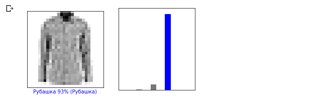
def plot_image(i, predictions_array, true_labels, images): predictions_array, true_label, img = predictions_array[i], true_label[i], images[i] plt.grid(False) plt.xticks([]) plt.yticks([]) plt.imshow(img[...,0], cmap=plt.cm.binary) predicted_label = np.argmax(predictions_array) if predicted_label == true_label: color = 'blue' else: color = 'red' plt.xlabel("{} {:2.0f}% ({})".format(class_names[predicted_label], 100 * np.max(predictions_array), class_names[true_label]), color=color) def plot_value_array(i, predictions_array, true_label): predictions_array, true_label = predictions_array[i], true_label[i] plt.grid(False) plt.xticks([]) plt.yticks([]) thisplot = plt.bar(range(10), predictions_array, color="#777777") plt.ylim([0, 1]) predicted_label = np.argmax(predictions_array) thisplot[predicted_label].set_color('red') thisplot[true_label].set_color('blue') Let's take a look at the 0th image, the result of the model prediction and the array of predictions.
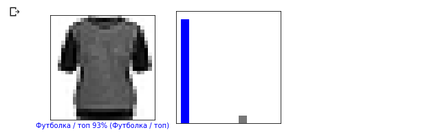
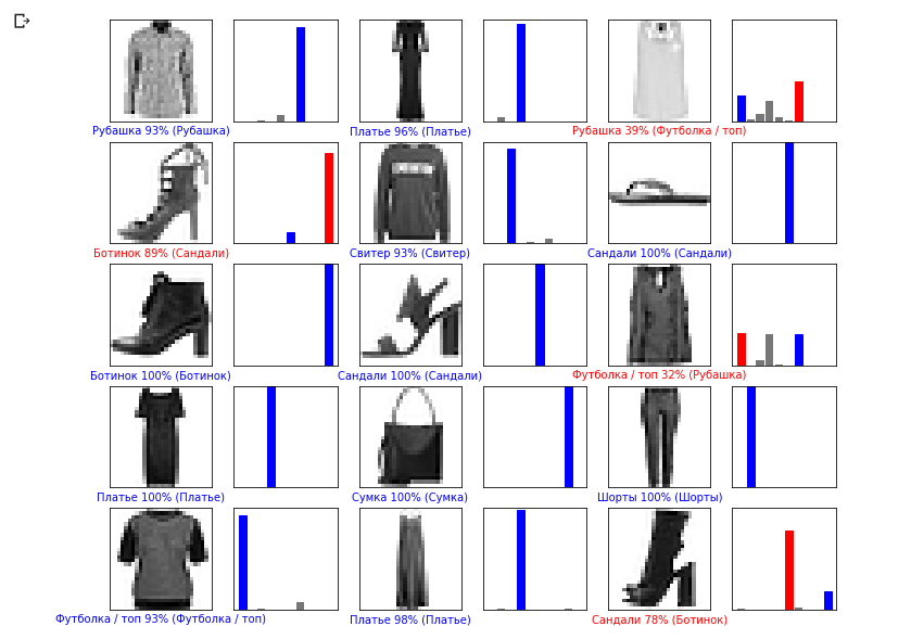
i = 0 plt.figure(figsize=(6,3)) plt.subplot(1,2,1) plot_image(i, predictions, test_labels, test_images) plt.subplot(1,2,2) plot_value_array(i, predictions, test_labels) i = 12 plt.figure(figsize=(6,3)) plt.subplot(1,2,1) plot_image(i, predictions, test_labels, test_images) plt.subplot(1,2,2) plot_value_array(i, predictions, test_labels) Let's now display some images with their respective predictions. Correct predictions are blue, incorrect ones are red. The value under the image reflects the percentage of confidence in the model that the input image corresponds to this class. Please note that the result may be incorrect even if the value of “confidence” is large.
num_rows = 5 num_cols = 3 num_images = num_rows * num_cols plt.figure(figsize=(2*2*num_cols, 2*num_rows)) for i in range(num_images): plt.subplot(num_rows, 2*num_cols, 2*i + 1) plot_image(i, predictions, test_labels, test_images) plt.subplot(num_rows, 2*num_cols, 2*i + 2) plot_value_array(i, predictions, test_labels) Use the trained model to predict the label for a single image:
img = test_images[0] print(img.shape) Conclusion:
(28, 28, 1) Models in
tf.kerasoptimized for prediction blocks (collections). Therefore, despite the fact that we use a single element, it is necessary to add it to the list: img = np.array([img]) print(img.shape) Conclusion:
(1, 28, 28, 1)Now let's predict the result:
predictions_single = model.predict(img) print(predictions_single) Conclusion:
[[3.1365438e-05 9.0029722e-08 5.0016833e-03 6.3597123e-05 6.8342514e-02 1.0856857e-08 9.2655218e-01 1.8982469e-09 8.4999692e-06 1.0296091e-09]] plot_value_array(0, predictions_single, test_labels) _ = plt.xticks(range(10), class_names, rotation=45) The model.predict method returns a list of lists (array of arrays), each for an image from a block of input data. We get the only result for our single input image:
np.argmax(predictions_single[0]) Conclusion:
6 As previously, the model predicted label 6 (shirt).
Exercises
Experiment with different models and see how the accuracy will change. In particular, try changing the following parameters:
- set the epochs parameter to 1;
- change the number of neurons in the hidden layer, for example, from a low value of 10 to 512 and see how the accuracy of the model prediction will change;
- add additional layers between the flatten-layer (smoothing layer) and the final dense-layer, experiment with the number of neurons on this layer;
- do not normalize pixel values and see what happens.
Do not forget to activate the GPU so that all the calculations are faster (
Runtime -> Change runtime type -> Hardware accelertor -> GPU). Also, if in the process of work you have any problems, then try to reset the global environment settings:Edit -> Clear all outputsRuntime -> Reset all runtimes
Degrees Celsius VS MNIST
- At this stage, we have already encountered two types of neural networks. Our first neural network has learned to convert degrees Celsius to degrees Frenheit, returning a single value that can be in a wide range of numerical values.
Our second neural network returns 10 probability values that represent the network’s confidence that the image fed to the input corresponds to a certain class.
Neural networks can be used to solve various kinds of problems.
The first class of problems that we solved with the prediction of a single value is called regression.. The conversion of degrees Celsius to degrees Fahrenheit is one example of the task of this class. Another example of this class of tasks may be the problem of determining the value of a house by room number, total area, location, and other characteristics.
The second class of problems, which we considered in this lesson by classifying images into existing categories, is called classification . According to the input data, the model will return the probability distribution (the “confidence” of the model that the input value belongs to this class). In this lesson, we developed a neural network that classified items of clothing into 10 categories, and in the next lesson we will learn to determine who the dog or cat is depicted in the photo, this task also applies to the classification task.
Let's summarize and note the difference between these two classes of problems - regression and classification .
Congratulations, you learned two types of neural networks! Get ready for the next lecture, where we will study a new type of neural networks - convolutional neural networks (CNN, convolutional neural networks).
Results
In this lesson, we taught the neural network to classify images with items of clothing. To do this, we used the MNIST Fashion dataset, which contains 70,000 images of clothing items. 60,000 of which we used to train the neural network, and the remaining 10,000 to test its performance. In order to feed these images to the input of our neural network, we needed to convert them (smooth out) from a 28x28 2D format to a 1D format of 784 elements. Our network consisted of a fully connected layer of 128 neurons and an output layer of 10 neurons, corresponding to the number of tags (classes, categories of elements of clothing). These 10 output values represented the probability distribution for each class. Softmax activation functioncounted the probability distribution.
We also learned about the differences between regression and classification .
- Regression : a model that returns a single value, for example, the value of a house.
- Classification : a model that returns a probability distribution among several categories. For example, in our problem with Fashion MNIST, the output values were 10 probability values, each of which was associated with a particular class (category of clothing item). I remind you that we used the softmax activation function just to get a probability distribution on the last layer.
Video version of the article
The video comes out a few days after publication and is added to the article.
... and standard call-to-action - subscribe, put a plus and share :)
YouTube
Telegram
In contact with
Source: https://habr.com/ru/post/454034/
All Articles