Maximum speed machine learning: Predictive Maintenance for four months

Author: Lyudmila Dezhkina, Solution Architect, DataArt

For about six months, our team has been working on the Predictive Maintenance Platform, a system that should predict possible errors and equipment failures. This direction is at the junction of IoT and Machine Learning, we have to work here with hardware and, in fact, with software. How we build Serverless ML with the Scikit-learn library on AWS will be discussed in this article. I will talk about the difficulties that we faced, and about the tools that are used, saved time.
')



This is how the requirements put forward by the customer from the very beginning

The interview with the client was difficult, basically we talked about machine learning, we were asked a lot about algorithms and specific personal experience. But I will not be shy - in this part we initially understand very well. The first stumbling block was a piece of Hardware, which contains the system. Still, my experience with iron is not so diverse.

The customer explained to us: “See, we have a pipeline.” A conveyor belt at the checkout in the supermarket immediately occurred to me. What and what can you teach there? But it quickly became clear that the whole sorting center with an area of ​​300–400 square meters was hidden behind the word conveyor. m, and in fact, there are many pipelines. That is, you need to connect with each other many pieces of equipment: sensors, robots. The classic illustration of the concept of "Industrial Revolution 4.0" , within which IoT and ML come together.

The topic of Predictive Maintenance will definitely be on the rise for at least another two to three years. Each conveyor is decomposed into elements: from a robot or a motor driving a conveyor belt to a separate bearing. At the same time, if any of these parts fail, the whole system stops, and in some cases the idle time of a conveyor can cost a million and a half dollars (this is no exaggeration!).

One of our customers is engaged in cargo transportation and logistics: on its base, robots unload 40 trucks in 8 minutes. There can be no delays here, the cars should come and go according to a very tight schedule, nobody repairs anything in the process of unloading. In general, on this base there are only two or three people with tablets. But there is a slightly different world, where everything looks not so fashionable, and where mechanics in gloves and without computers are directly on the site.

Our first small prototype project consisted of about 90 sensors, and everything went fine until the project had to be scaled. To equip the smallest separate part of the real sorting center, sensors require about 550 already.

PLC and sensors

Programmable logic controller - a small computer with a built-in cyclic program - most often used to automate the process. Actually, with the help of PLC, we take readings from the sensors: for example, acceleration and speed, voltage level, vibration along the axes, temperature (in our case - 17 indicators). The sensors are often wrong. Although our project is more than 8 months old, we still have our own laboratory where we experiment with sensors, selecting the most suitable models. Now, for example, we are considering the possibility of using ultrasonic sensors.

Personally, I first saw the PLC, only when I got on the customer’s site. As a developer, I had never encountered them before, and it was rather unpleasant: as soon as we went further in conversation, two, three, and four-phase motors, I began to lose the thread. Approximately 80% of the words were still understandable, but the general meaning stubbornly eluded. In general, this is a serious problem, the roots of which are at a rather high threshold for entering the PLC programming - such a microcomputer, where you can really do something, costs at least 200–300 dollars. The programming itself is simple, and problems begin only when the sensor is attached to a real conveyor or motor.



Standard set of sensors "37 in 1"

Sensors, as you know, are different. The simplest ones we managed to find cost from $ 18. The main characteristic is “bandwidth and resolution” - how much data the sensor transmits per minute. From my own experience, I can say that if a manufacturer claims, say, 30 datapot per minute, in reality their number is unlikely to be more than 15. And this also has a serious problem: the topic is fashionable, and some companies are trying to capitalize on this hype. We tested the sensors at a cost of $ 158, the bandwidth of which theoretically allowed us to simply throw out a part of our code. But in actual fact, they turned out to be an absolute analogue of those devices for $ 18 apiece.

The first stage: we fix the sensors, collect data

Actually, the first phase of the project was to install hardware, the installation itself was a long and tedious process. This is also a whole science - how you attach the sensor to a motor or box may depend on the data that it eventually collects. We had a case where one of two identical sensors was attached inside the box, and the other outside. Logic suggests that inside the temperature should be higher, but the collected data suggested the opposite. It turned out that the system failed, but when the developer arrived at the factory, he saw that the sensor was not just in the box, but directly on the fan located there.



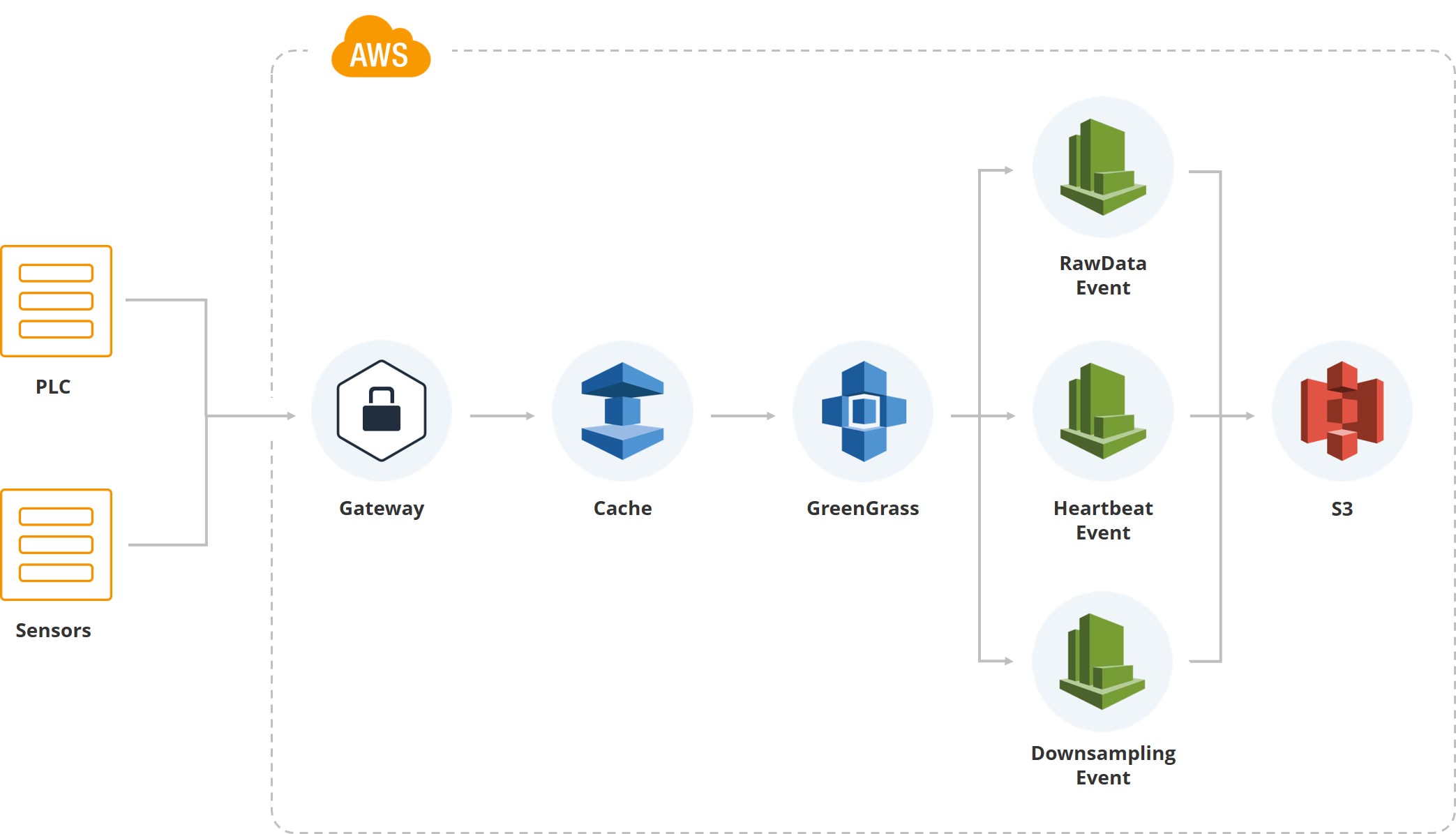
This illustration shows how the first data entered the system. We have a gateway, there are PLC and sensors associated with it. Then, of course, cash - equipment usually works on mobile cards and all data is transmitted via the mobile Internet. Since one of the customer’s sorting centers is located in an area where there are often hurricanes, and the connection can break, we accumulate data on the gateway until it is restored.

Next we use the Greengrass service from Amazon, which lets the data inside the cloud system (AWS).

Once the data is inside the cloud, a bunch of events are triggered. For example, we have an event for raw data, which saves file system data. There is a “heartbeat” to indicate the normal operation of the system. There is a “downsampling”, which is used for showing on the UI, and for processing (take the average value, say, per minute for a particular indicator). That is, besides the raw data, we have downsampled data that falls on the screens of users who monitor the system.

Raw data is stored in parquet format. At first we chose JSON, then we tried CSV, but in the end we came to the conclusion that it was the “parquet” that satisfied both the analytics team and the development team.

Actually, the first version of the system was built on DynamoDB, and I don’t want to say anything bad about this database. Simply, as soon as we had analysts — mathematicians who must work with the data — it turned out that the query language for DynamoDB was too complicated for them. They had to specially prepare data for ML and analytics. Therefore, we stopped at Athena - the query editor in AWS. For us, its advantages are that it allows you to read Parquet data, write SQL, and collect the results in a CSV file. Just what the analyst team needs.

Stage two: what do we analyze?

So, from one small object we collected about 3 GB of raw data. Now we know a lot about temperature, vibration and acceleration along the axes. It means that the time has come for our mathematicians to come together to understand how, in fact, what we are trying to predict on the basis of this information.

The goal is to minimize equipment downtime.



People enter this Coca-Cola plant only when they receive a signal of breakage, oil leakage or, say, a puddle on the floor. The cost of one robot starts at $ 30,000 dollars, but almost all production is built on them



About 10,000 people work at six Tesla factories, and for production of such a scale it is quite a bit. Interestingly, Mercedes plants are automated to a much greater extent. It is clear that all robots involved need constant monitoring.

The more expensive the robot, the less its working part vibrates. With simple actions, this may not be decisive, but more subtle operation, say, with the neck of the bottle, requires that it be kept to a minimum. Of course, the vibration level of expensive cars must be constantly monitored.

Time-saving services

We launched the first installation in just over three months, and I believe that this is fast.



Actually, these are the main five points, which allowed to save developer efforts

The first, due to which we have reduced the time - most of the system is built on AWS, which scales on its own. As soon as the number of users exceeds a certain threshold, auto-scaling works, and no one from the team has to spend time on it.

I would like to draw attention to two nuances. First, we work with large amounts of data, and in the first version of the system we had pipelines in order to make backups. After some time, the data became too much, and keeping copies for them became too expensive. Then we simply left Raw data lying in the bucket, read-only, forbidding them to be deleted, and refused backups.

Our system involves continuous integration, to support the new site and the new installation takes not so much time.

It is clear that realtime is built on events. Although, of course, there are difficulties due to the fact that some events are triggered twice or the system loses touch, for example, due to weather conditions.

Data encryption, which the customer required, automatically takes place in AWS. Each client has its own bake, and we don’t do anything to encrypt data.

Meeting with analysts

We received the very first code in PDF format along with the request to implement this or that model. While we did not start receiving the code in the form of .ipynb, it was alarming, but the fact is that analysts are mathematicians far from programming. All our operations take place in the cloud, we do not allow downloading data. Together, all these moments pushed us to try the SageMaker platform.

SageMaker allows out of the box to use about 80 algorithms, it includes frameworks: Caffe2, Mxnet, Gluon, TensorFlow, Pytorch, Microsoft cognitive tool kit. We currently use Keras + TensorFlow, but all but the Microsoft cognitive toolkit have had time to try. Such wide coverage allows us not to limit our own analytical team.



For the first three or four months, all the work was done by people with the help of simple mathematics; no ML really existed yet. Part of the system is based on purely mathematical laws, and it is designed for statistical data. That is, we monitor the average temperature level, and if we see that it goes off scale, alerts will be triggered.

Then follows the training model. Everything looks easy and simple, and it seems so before the start of implementation.

Build, train, deploy ...

Briefly tell you how we got out of the situation. Look at the second column: collect data, process, clean, use S3 bucket and Glue to launch events and create “partitions”. We have all the data decomposed into partitions for Athena, this is also an important nuance, because Athena is built on top of S3. Athena itself is very cheap. But we pay for what we read the data and get them from S3, t. H. Each request can be very expensive. Therefore, we have a large partitions system.

We have a downsampler. And Amazon EMR, which allows you to quickly collect data. Actually, for feature engineering in our cloud, for every analyst, Jupyter Notebook is raised - this is their own instance. And they analyze everything directly in the cloud.

Thanks to SageMaker, we were primarily able to skip the Training Clusters stage. If we didn’t use this platform, we would have to raise clusters in Amazon, and some of the DevOps engineers would have to keep an eye on them. SageMaker allows you to raise a cluster using the parameters of the method on the Docker image, you just have to specify the number of instances in the parameter you want to use.

Next, we do not have to do scaling. If we want to process a large algorithm or we need to urgently calculate something, we turn on auto-scaling (everything depends on whether you want to use a CPU or a GPU).

In addition, all our models are encrypted: it also goes out of the box in SageMaker - the binaries that are in S3.

Model Deployment

We are getting to the first model, deployed in the environment. Actually, SageMaker allows you to save model artifacts, but just at this stage we had a lot of controversy, because SageMaker has its own model format. We wanted to get away from it, getting rid of restrictions, so our models are stored in pickle format, so that if we want we can use at least Keras, even TensorFlow or something else. Although we used the first model from SageMaker, as it is, through the native API.

SageMaker makes it easy to work in three more steps. Every time you try to predict something, you have to start some process, give the data and get the prediction values. With this, everything went fine until you needed custom algorithms.



Analysts know that they have a CI and a repository. In the CI repository there is a folder where they should upload three files. Serve.py is a file that allows SageMaker to raise the Flask service and communicate with SageMaker itself. Train.py— class with the train method, in which they have to put everything they need for a model. Finally, predict.py - with its help they raise this class, within which there is a method. Having access, they bring up all sorts of resources from S3 - inside SageMaker we have an image that allows you to run anything from the interface and programmatically (we do not limit them).

From SageMaker we get access to predict.py - inside image - it’s just an application on Flask that allows you to call predict or train with certain parameters. All this is tied to S3 and, in addition, they have the ability to save models from Jupyter Notebook. That is, in Jupyter Notebook, analysts have access to all the data, and they can do some kind of experiment.

In production, it all falls as follows. We have users, there is a predict values ​​endpoint. The data lie on S3 and get Athena. Every two hours, an algorithm is launched that counts the prediction for the next two hours. Such a time step is due to the fact that in our case, about 6 hours of analytics are enough to say that something is wrong with the motor. Even at the moment of switching on, the motor heats up for 5–10 minutes, and there are no sharp jumps.

In systems that are critical, for example, when Air France checks the turbines of an aircraft, the prediction is done at the rate of 10 minutes. In this case, the accuracy is 96.5%.

If we see that something is going wrong, the notification system is activated. Then someone from the set of users on the clock or another device receives a notification that a particular motor behaves abnormally. He goes and checks his condition.

Manage Notebook Instances

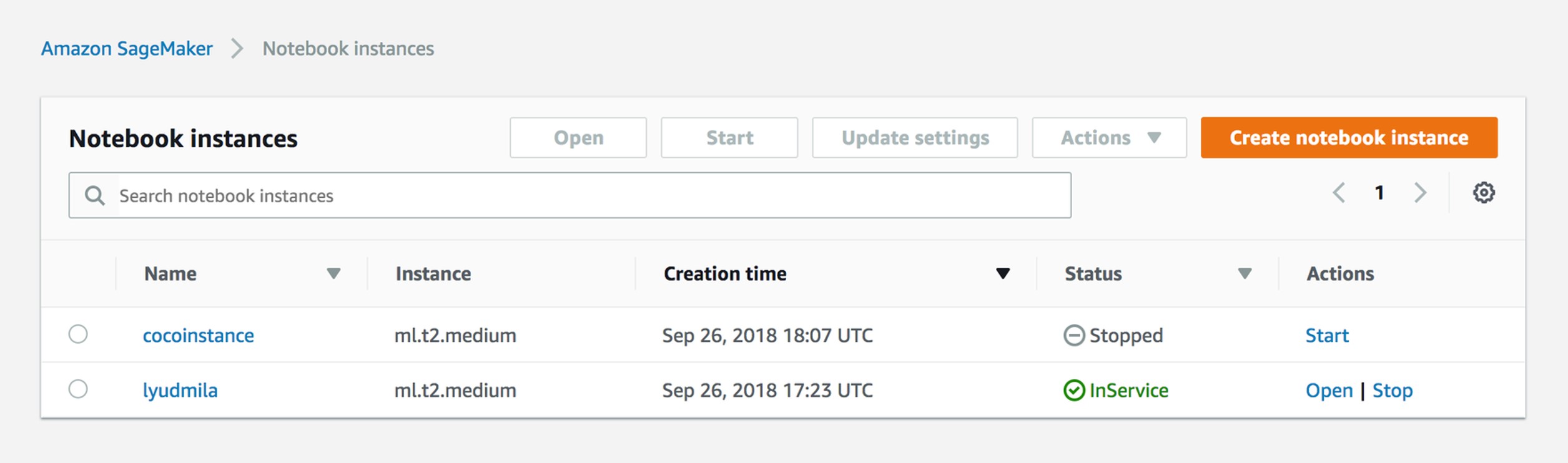
In fact, everything is very simple. Coming to work, the analyst runs the instance on Jupyter Notebook. He gets the role and session, so two people cannot edit the same file. Actually, we now have an instance for each analyst.

Create Training Job

SageMaker has an understanding of training jobs. Its result, if you use just an API - a binary that is stored on S3: from the parameters you provide, your model is obtained.

sagemaker = boto3.client('sagemaker') sagemaker.create_training_job(**create_training_params) status = sagemaker.describe_training_job(TrainingJobName=job_name)['TrainingJobStatus'] print(status) try: sagemaker.get_waiter('training_job_completed_or_stopped').wait(TrainingJobName=job_name) finally: status = sagemaker.describe_training_job(TrainingJobName=job_name)['TrainingJobStatus'] print("Training job ended with status: " + status) if status == 'Failed': message = sagemaker.describe_training_job(TrainingJobName=job_name)['FailureReason'] print('Training failed with the following error: {}'.format(message)) raise Exception('Training job failed') 

Training Params Example

 { "AlgorithmSpecification": { "TrainingImage": image, "TrainingInputMode": "File" }, "RoleArn": role, "OutputDataConfig": { "S3OutputPath": output_location }, "ResourceConfig": { "InstanceCount": 2, "InstanceType": "ml.c4.8xlarge", "VolumeSizeInGB": 50 }, "TrainingJobName": job_name, "HyperParameters": { "k": "10", "feature_dim": "784", "mini_batch_size": "500", "force_dense": "True" }, "StoppingCondition": { "MaxRuntimeInSeconds": 60 * 60 }, "InputDataConfig": [ { "ChannelName": "train", "DataSource": { "S3DataSource": { "S3DataType": "S3Prefix", "S3Uri": data_location, "S3DataDistributionType": "FullyReplicated" } }, "CompressionType": "None", "RecordWrapperType": "None" } ] } 

Options. The first is the role: you must specify what your SageMaker instance has access to. That is, in our case, if the analyst works with two different productions, he should see one bucket and not see the other. Output config is where you save all the metadata of the model.

We skip the autoscale and we can simply indicate the number of instances where you want to run this training job. At first, we generally used middle instances without TensorFlow or Keras, and that was enough.

Hyperparameters. You specify the Docker image in which you want to run. Amazon usually provides a list of algorithms and images with them, that is, you must specify hyperparameters - the parameters of the algorithm itself.

Create Model

 %%time import boto3 from time import gmtime, strftime job_name = 'kmeans-lowlevel-' + strftime("%Y-%m-%d-%H-%M-%S", gmtime()) print("Training job", job_name) from sagemaker.amazon.amazon_estimator import get_image_uri image = get_image_uri(boto3.Session().region_name, 'kmeans') output_location = 's3://{}/kmeans_example/output'.format(bucket) print('training artifacts will be uploaded to: {}'.format(output_location)) create_training_params = \ { "AlgorithmSpecification": { "TrainingImage": image, "TrainingInputMode": "File" }, "RoleArn": role, "OutputDataConfig": { "S3OutputPath": output_location }, "ResourceConfig": { "InstanceCount": 2, "InstanceType": "ml.c4.8xlarge", "VolumeSizeInGB": 50 }, "TrainingJobName": job_name, "HyperParameters": { "k": "10", "feature_dim": "784", "mini_batch_size": "500", "force_dense": "True" }, "StoppingCondition": { "MaxRuntimeInSeconds": 60 * 60 }, "InputDataConfig": [ { "ChannelName": "train", "DataSource": { "S3DataSource": { "S3DataType": "S3Prefix", "S3Uri": data_location, "S3DataDistributionType": "FullyReplicated" } }, "CompressionType": "None", "RecordWrapperType": "None" } ] } sagemaker = boto3.client('sagemaker') sagemaker.create_training_job(**create_training_params) status = sagemaker.describe_training_job(TrainingJobName=job_name)['TrainingJobStatus'] print(status) try: sagemaker.get_waiter('training_job_completed_or_stopped').wait(TrainingJobName=job_name) finally: status = sagemaker.describe_training_job(TrainingJobName=job_name)['TrainingJobStatus'] print("Training job ended with status: " + status) if status == 'Failed': message = sagemaker.describe_training_job(TrainingJobName=job_name)['FailureReason'] print('Training failed with the following error: {}'.format(message)) raise Exception('Training job failed') %%time import boto3 from time import gmtime, strftime model_name=job_name print(model_name) info = sagemaker.describe_training_job(TrainingJobName=job_name) model_data = info['ModelArtifacts']['S3ModelArtifacts'] print(info['ModelArtifacts']) primary_container = { 'Image': image, 'ModelDataUrl': model_data } create_model_response = sagemaker.create_model( ModelName = model_name, ExecutionRoleArn = role, PrimaryContainer = primary_container) print(create_model_response['ModelArn']) 

Creating a model is the result of a training job. After the last one is completed, and when you monitor it, it is saved on S3, and you can use it.



That's how it looks from the perspective of analysts. Our analysts come to the models, and they say: I want to launch this model in this image. They simply point to the S3 folder, Image, and enter parameters into the GUI. But there are nuances and difficulties, so we switched to custom algorithms.

Create Endpoint

 %%time import time endpoint_name = 'KMeansEndpoint-' + strftime("%Y-%m-%d-%H-%M-%S", gmtime()) print(endpoint_name) create_endpoint_response = sagemaker.create_endpoint( EndpointName=endpoint_name, EndpointConfigName=endpoint_config_name) print(create_endpoint_response['EndpointArn']) resp = sagemaker.describe_endpoint(EndpointName=endpoint_name) status = resp['EndpointStatus'] print("Status: " + status) try: sagemaker.get_waiter('endpoint_in_service').wait(EndpointName=endpoint_name) finally: resp = sagemaker.describe_endpoint(EndpointName=endpoint_name) status = resp['EndpointStatus'] print("Arn: " + resp['EndpointArn']) print("Create endpoint ended with status: " + status) if status != 'InService': message = sagemaker.describe_endpoint(EndpointName=endpoint_name)['FailureReason'] print('Training failed with the following error: {}'.format(message)) raise Exception('Endpoint creation did not succeed') 

So much code is needed to create an Endpoint that jerks from any lambda and from the outside. Every two hours we have an event that jerks Endpoint.

Endpoint View

So analysts see it. They simply indicate the algorithm, time and pull it with the hands from the interface.

Invoke endpoint

 import json payload = np2csv(train_set[0][30:31]) response = runtime.invoke_endpoint(EndpointName=endpoint_name, ContentType='text/csv', Body=payload) result = json.loads(response['Body'].read().decode()) print(result) 

And this is how it is done from lambda. That is, we have Endpoint inside, and every two hours we send a payload in order to make a prediction.

Useful SageMaker Links: links to github

These are very important links. Honestly, after we started using the usual Sagemaker GUI, everyone understood that sooner or later we would come to the custom algorithm, and all this would be assembled by hand. These links can be used to find not only the use of algorithms, but also the assembly of custom images:

github.com/awslabs/amazon-sagemaker-examples

github.com/aws-samples/aws-ml-vision-end2end

github.com/juliensimon

github.com/aws/sagemaker-spark

What's next?

We have come to the fourth production and now, apart from analytics, we have two ways of development. First, we are trying to get logs from the mechanics, that is, we are trying to come to the training with support. The first Mantainence logs that we received look like this: something broke on Monday, I went there on Wednesday, started repairing it on Friday. We are now trying to deliver a CMS to the customer - a content management system that will allow logging breakdown events.

How it's done? As a rule, as soon as a breakdown happens, the mechanic comes in and changes the part very quickly, but he can fill out all paper forms, say, in a week. By this time, the person simply forgets what exactly happened to the part. CMS, of course, takes us to a new level of interaction with the mechanics.

Secondly, we are going to install ultrasonic sensors on the motors, which read the sound and are engaged in spectral analysis.

It is possible that Athena will give up, because on large data, using S3 is expensive. At the same time, Microsoft recently announced its own services, and one of our customers wants to try to do roughly the same thing already on Azure. Actually, one of the advantages of our system is that it can be disassembled and assembled elsewhere, like from cubes.