Hello everyone, I work as a research programmer in the Mail.ru Group computer vision team. By the Victory Day this year, we decided to make a project for the restoration of military photographs . What is photo restoration? It consists of three stages:

• we find all the defects of the image: breaks, abrasions, holes;
  
• paint over defects found based on pixel values ​​around them;
  
• color the image.
  

In this article, I will go through each of the restoration stages in detail and tell you how and where we took the data, what networks we were taught, what happened to us, what rake we stepped on.

Defect Search

We want to find all the pixels related to the defects in the loaded photo. First we need to understand what photos of the war years people will upload. We turned to the organizers of the project "Immortal Regiment", who shared data with us. After analyzing them, we noticed that people often load portraits, single or group, with moderate or large number of defects.
')
Then it was necessary to collect a training set. The training set for the segmentation task is an image and a mask on which all defects are marked. The easiest way is to put photos in markup to assessors. Of course, people can find defects well, but the problem is that the markup is a very long process.



It can take from one hour to a full working day to markup pixels related to defects in a single photo, so for several weeks it is difficult to collect a sample of more than 100 photos. Therefore, we tried to somehow complement our data and wrote the defects ourselves: we took a clean photo, put artificial defects on it and got a mask showing us exactly which parts of the image were defective. The main part of our training sample was 79 photos, marked up manually, of which we transferred 11 pieces to the test sample.

The most popular approach for the segmentation task: take Unet with a pre-trained encoder and minimize the amount $$$Bce$( binary cross-entropy ) and $$$DICE$( Sørensen – Dice coefficient ).

What problems arise with this approach in the problem of segmentation of defects?

• Even if it seems to us that there are a lot of defects in a photo, that it is very dirty and is heavily battered by time, the area occupied by defects is still much less than the intact part of the image. To solve this problem, you can increase the weight of the positive class in $$$Bce$, and the optimal weight will be the ratio of the number of all pure pixels to the number of pixels belonging to defects.
  
• The second problem is that if we use Unet from the box with a pre-trained encoder, for example Albunet-18, then we lose a lot of positional information. The first layer of Albunet-18 consists of a convolution with core 5 and stride equal to two. This allows the network to work quickly. We sacrificed the network time for better localization of defects: removed the max pooling after the first layer, reduced the stride to 1 and reduced the core of the bundle to 3.
  
• If we work with small images, for example, compressing the image to 256 x 256 or 512 x 512, then small defects will simply disappear due to interpolation. Therefore, you need to work with a large picture. Now in production, we are segmenting the defects in a 1024 x 1024 photograph. Therefore, it was necessary to train the neural network on large numbers of large images. And because of this, there are problems with a small batch size on a single video card.
  
• During training, we have about 20 pictures per one card. Because of this, the estimate of the mean and variance in the BatchNorm layers is inaccurate. In-place BatchNorm helps us solve this problem, which, firstly, saves memory, and secondly, it has a version of Synchronized BatchNorm, which synchronizes statistics between all the cards. Now we consider the mean and variance not for 20 pictures on one card, but for 80 pictures with 4 cards. This improves network convergence.
  

In the end, increasing the weight $$$Bce$By changing the architecture and using In-place BatchNorm, we began to look for defects in the photo. But cheaply you could have done a little better by adding Test Time Augmentation. We can drive the network once on the input image, then mirror it and drive the network again, this can help us find small defects.



As a result, our network converged on four GeForce 1080Ti in 18 hours. Inference takes 290 ms. It turns out long enough, but it is a payment that we well look for small defects. Validation $$$DICE$equal to 0.35, and $$$ROCAUC$- 0.93.

Restoration of fragments

Unet helped us solve this problem again. At the entrance we gave him the original image and a mask, on which we mark the spaces with pure units, and the zeroes - those pixels that we want to paint over. We collected the data as follows: we took from the Internet a large dataset with pictures, for example, OpenImagesV4, and artificially added defects that are similar in shape to those found in real life. And after that they trained the network to restore the missing parts.

How can we modify Unet for this task?

You can use Partial Convolution instead of the usual convolution. Her idea is that when we collapse a region of a picture with some kind of core, we do not take into account the pixel values ​​related to defects. This helps make the fill more accurate. An example from an NVIDIA article . In the central picture, they used Unet with the usual convolution, and on the right - with Partial Convolution:



We trained the network for 5 days. On the last day, we froze BatchNorm, which helped to make the borders of the part of the image being painted over less visible.

The network processes 512 x 512 images in 50 ms. Validation PSNR is 26.4. However, in this task, you cannot completely trust metrics. Therefore, we first chased several good models on our data, anonymized the results, and then voted for those that we liked more. So we chose the final model.

I mentioned that we artificially added defects to clean images. When training, you need to very carefully monitor the maximum size of the superimposed defects, because with very large defects that the network has never seen in the training process, it will wildly fantasize and give an absolutely inapplicable result. So, if you need to paint over large defects, when training, also submit large defects.

Here is an example of the algorithm:

Coloring

We have segmented defects and painted them, the third step is color reconstruction. Let me remind you that among the photos of the "Immortal Regiment" there are a lot of single or group portraits. And we wanted our network to work well with them. We decided to make our colorization, because none of the services we know paints portraits quickly and well.



GitHub has a popular repository for coloring photos. On average, he does the job well, but he has a few problems. For example, he loves to paint clothes in blue. Therefore, we also rejected it.

So, we decided to make a neural network for colorization. The most obvious idea is to take a black and white image and predict three channels, red, green and blue. But, generally speaking, we can simplify our work. We can work not with the RGB color representation, but with the YCbCr representation. The Y component is brightness (luma). The downloaded black and white image is the Y channel, we will reuse it. It remained to predict Cb and Cr: Cb is the difference of blue color and brightness, and Cr is the difference of red color and brightness.



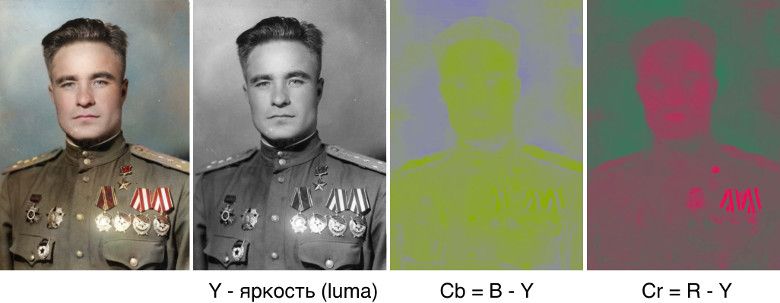
Why did we choose the YCbCr representation? The human eye is more susceptible to changes in brightness than to changes in color. Therefore, we reuse the Y-component (brightness), something to which the eye is initially well susceptible, and we predict Cb and Cr, in which we can make a little more mistake, because the person is less “false” in colors. This feature began to actively use at the dawn of color television, when the channel capacity was not enough to transmit all the colors completely. The image was transferred to YCbCr, transferred to the Y-component without changes, and Cb and Cr were compressed twice.

How to build a baseline

You can again take Unet with a pre-trained encoder and minimize L1 Loss between real CbCr and predicted. We want to paint portraits, so besides the photos from OpenImages, we need to add photos specific to our task.

Where can I get color photos of people in uniform? There are people on the Internet who paint old photos as a hobby or to order. They do this very carefully, trying to fully observe all the nuances. Painting the form, shoulder straps, medals, they turn to archival materials, so the result of their work can be trusted. In total, we used 200 hand-painted photos. The second useful source of data is the site of the Workers 'and Peasants' Red Army . One of its creators was photographed in almost all possible variants of the military uniform of the Great Patriotic War.



In some photographs, he repeated the poses of people from famous archival photographs. It is especially good that it was shot on a white background, it allowed us to augment data very well, adding different natural objects to the background. We also used ordinary modern portraits of people, complementing them with signs of distinction and other attributes of wartime clothing.

We trained AlbuNet-50 - this is Unet, which uses AlbuNet-50 as an encoder. The network began to produce adequate results: the skin is pink, the eyes are gray-blue, and the epaulets are yellowish. But the problem is that she painted the pictures in spots. This is due to the fact that from the point of view of the L1 error, it is sometimes more profitable not to do anything than to try to predict a certain color.


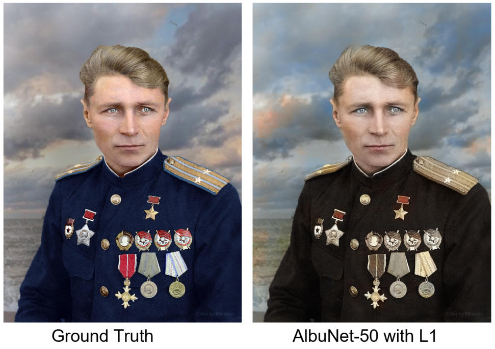
We are comparing our result with a photo of Ground Truth - the artist’s hand- colored coloring under the nickname Klimbim

How to solve this problem? We need a discriminator: a neural network, which we will input images to the input, and it will tell you how realistic this image looks. Below one photo is painted by hand, and the second is neural network. What do you think, what?




As a discriminator, we use the discriminator from the Self-Attention GAN article. This is a small convolutional network, in the last layers of which the so-called Self-Attention is embedded. It allows you to "pay attention" to the details of the image. We also use spectral normalization. Exact explanation and motivation can be found in the article. We trained the network with a combination of L1-loss and the error returned by the discriminator. Now the network better paints the details of the image, and the background will be more consistent. Another example: on the left, the result of a network trained only with L1-loss, on the right — with L1-loss and a discriminator error.



On four Geforce 1080Ti training took two days. The network worked for 30 ms in the picture 512 x 512. Validation MSE - 34.4. As in the inpainting task, metrics can be not completely believed. Therefore, we selected 6 models that had the best metrics for validation, and blindly voted for the best model.

After rolling out the model in production, we continued the experiments and came to the conclusion that it is better to minimize not per-pixel L1-loss, but perceptual loss. To calculate it, you need to drive the network prediction and the original photo through the VGG-16 network, take the feature maps on the lower layers and compare them by MSE. This approach paints more areas and helps to get a more colorful picture.

Conclusions and Conclusion

Unet is a cool model. In the first task of segmentation, we encountered a problem when learning and working with high-resolution pictures, so we use In-Place BatchNorm. In the second task (Inpainting) instead of the usual convolution, we used Partial Convolution, this helped to achieve better results. In the colorization task to Unet, we added a small discriminator network that penalized the generator for an unrealistic-looking image and used perceptual loss.

The second conclusion - assessments are important. And not only at the stage of marking pictures before training, but also to validate the final result, because in the tasks of painting over defects or colorization, you still need to validate the result with the help of a person. We give the user three photos: the original one with the defects removed, colorized with the defects removed and just the colorized photo in case the algorithm for searching and painting defects is wrong.

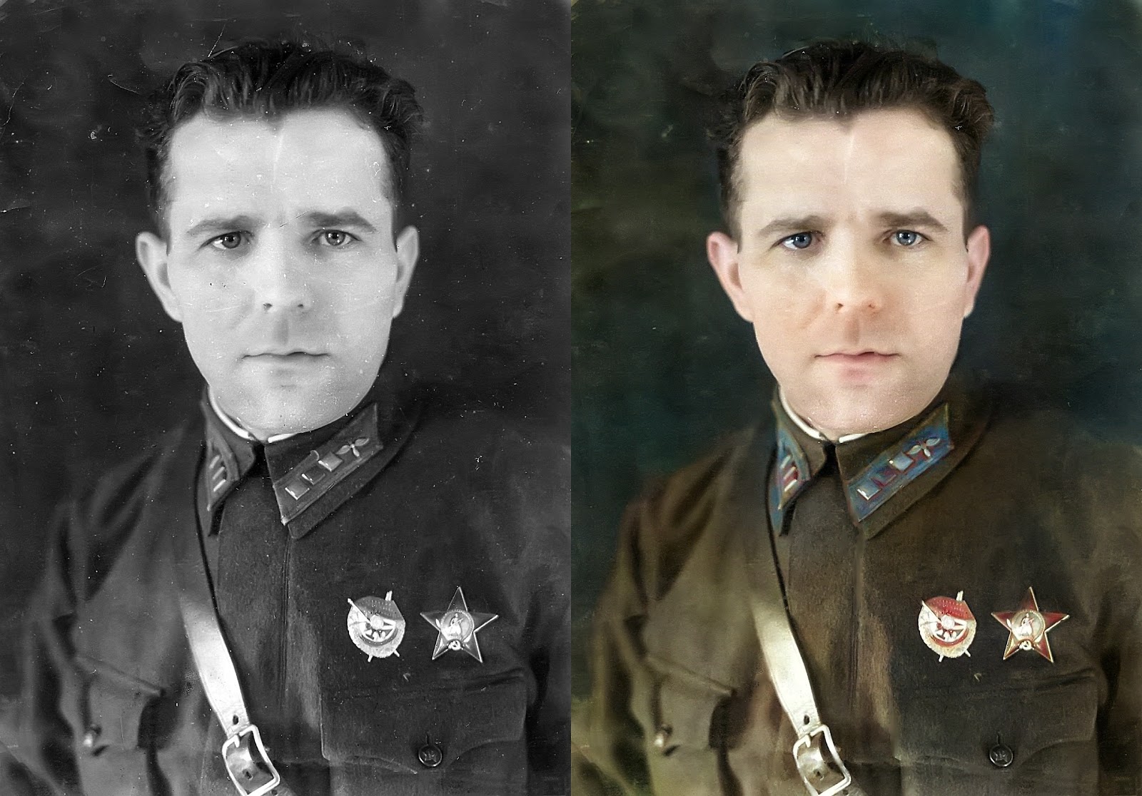
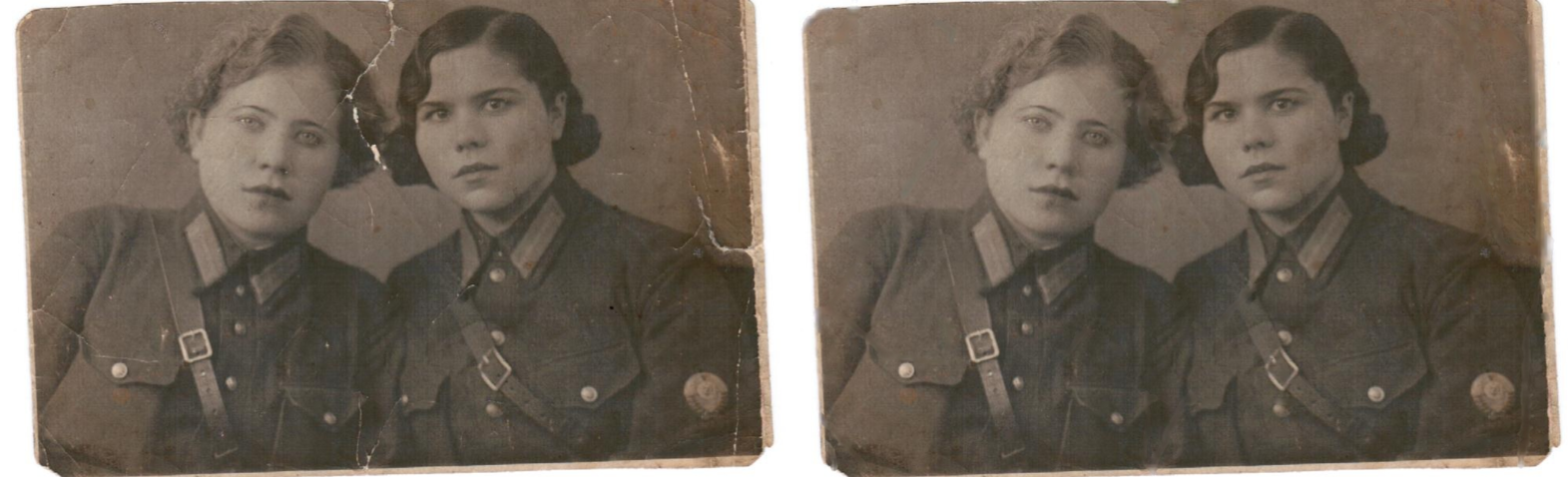
We took some photos of the War Album project and processed them with our neural networks. Here are the results obtained:



And here you can see them in the original resolution and at each stage of processing.